Genetic Drift in Genetic Algorithm Selection
Schemes
Alex Rogers and Adam Pr¨
ugel-Bennett
ISIS Research Group
Department of Electronics and Computer Science
University of Southampton
Highfield, Southampton, SO17 1BJ
England
[email protected]
Abstract— A method for calculating genetic drift in terms of changing population fitness variance is presented. The method allows for an easy comparison of different selection schemes and exact analytical results are derived for tra-ditional generational selection, steady-state selection with varying generation gap, a simple model of Eshelman’s CHC algorithm, and (μ+λ) evolution strategies. The effects of changing genetic drift on the convergence of a GA are demonstrated empirically.
Keywords— Genetic Drift, Selection Operator, Genetic Al-gorithm, Evolution Strategy
I. Introduction
G
ENETIC drift is a term borrowed from populationge-netics where it is used to explain changes in gene fre-quency through random sampling of the population. It is a phenomenon observed in genetic algorithms (GA) due to the stochastic nature of the selection operator, and is one of the mechanisms by which the population converges to a single member. Analysis of genetic drift is often per-formed by calculating the Markov chain transition matrices and hence finding the time for the system to reach an ab-sorption state where all population members are identical. Comparisons in the genetic algorithm literature are often performed numerically in this fashion [1], [2]. In population genetics some work has been to done to solve this analyt-ically [3], [4], [5] however the results are approximations and are difficult to generalise to other cases.
Analysis of selection schemes such as those by Pr¨
ugel-Bennett and Shapiro [6], [7], [8], Rattray [9] and
M¨uhlenbein [10] show that the change in mean fitness at
each generation is a function of the population fitness vari-ance. At each generation this variance is reduced due to two factors. One factor is selection pressure producing mul-tiple copies of fitter population members whilst the other factor is independent of population member fitness and is due to the stochastic nature of the selection operator — genetic drift. The loss in population fitness variance due to genetic drift thus has a direct effect on the performance of the genetic algorithm. By considering neutral selection we decouple the effect of selection pressure and can see the effect of genetic drift directly.
This paper presents a method of calculating the rate of genetic drift in terms of this change in population fitness
variance. Unlike calculations in terms of convergence time, this approach lends itself to an exact analytical solution. We are able to derive a general expression for the change in population fitness variance due to genetic drift and apply it to the range of selection schemes used in evolutionary al-gorithms. We first consider the generational GA and then compare it to steady-state selection where one member is drawn from the population, replicated, and replaces an-other population member chosen at random.
To generalise between these two extremes, De Jong [1], [11] introduced the termgeneration gap,G, which describes the percentage of the population selected from the initial population at each time step. For generational selection
G= 1 and for steady-state selectionG= 1/P. We follow
this generalisation and calculate the change in variance for any value of generation gap.
The formalism can also be extended to other non tradi-tional selection schemes such as that used in Eshelman’s CHC algorithm [12]. Here we confirm analytically an
ob-servation made by Schaffer et al. [2] that shows using a
numerical Markov chain analysis that a simple model of CHC style selection exhibits half the rate of genetic drift of the traditional genetic algorithm. The simple model of the CHC algorithm is equivalent to selection schemes in evolution strategies and we can generalise the approach for these selection schemes.
In Section II we derive the result which enables us to calculate the rate of genetic drift. In Section III we present the analytical results for different selection schemes and compare them to simulation results. Section IV contains details of the calculations and in Section V we discuss the results and their implications on the performance of genetic algorithms.
II. Population Fitness Variance
If we consider an initial population of P discrete
mem-bers each with fitnessFα, the variance (κ2) of the popula-tion fitness distribupopula-tion is simply given by,
κ2 = EF2−E[F]2
= 1
P
P
α=1
F2 α−
1 P
P
α=1
Fα
2
We can separate out terms that are not independent to give,
κ2=
1 P − 1 P2 P α=1 F2 α− 1 P2
α=β
FαFβ. (2)
We now apply some selection scheme to this population
and draw from it a new population of P individuals. In
this new population there are nownαcopies of population
memberFαand the variance of the new population fitness
distribution is given by,
κ 2 = 1 P P α=1
nαFα2−
1 P P α=1
nαFα
2
. (3)
Again we can separate out terms that are not independent,
κ 2= P α=1 nα P − n2 α P2 F2 α−
α=β
nαnβ
P2 FαFβ. (4)
To consider the average case, we average over all ways of performing selection. In the case of neutral selection, nα
is independent of Fα and these terms may be taken
out-side the summation and the expected population fitness variance considered,
E[κ2] =
E[n] P −
En2
P2
P
α=1
F2
α−E[nPα2nβ]
α=β
FαFβ. (5)
To simplify this result further, we use the fact that popu-lation size is kept constant and thusE[n] = 1. We can use this to derive the identity,
P
α=1
nα
2
=P2=
P α=1 n2 α+
α=β
nαnβ. (6)
Averaging over all possible selections gives,
P2=PEn2+P(P−1)E[n
αnβ], (7)
and thus,
E[nαnβ] = P−E
n2
P−1 . (8)
Substituting this expression into eqn. (5) gives,
E[κ2] = P−E
n2
P−1
⎡ ⎣1
P − 1 P2 P α=1 F2 α−P12
α=β
FαFβ
⎤ ⎦. (9)
The term within the square brackets is simply the fitness variance of the initial population given in eqn. (2) and thus,
E[κ2] =P−E
n2
P−1 κ2. (10)
We can find the change in population fitness variance for
any selection scheme simply by calculating En2 — the
expected square of the number of times any population member is selected. This is related to the variance in the number of times any member is selected —V[n]. AsV[n] =
En2−E[n]2, we can rewrite eqn. (10) in these terms, E[κ2] =
1− V[n] P−1
κ2. (11)
This expression is the basis for the results derived in this paper. It describes the change in population fitness vari-ance due to selection, genetic drift, in terms of the varivari-ance in the number of times any individual is selected.
III. Results
The change in the population fitness variance due to se-lection, genetic drift, is dependent only on the variance of the number of times any individual population member is selected -V[n]. If we select each population member once and only once thenV[n] = 0 and our expression in eqn. (11) is equal to one. As expected we see no change in population variance — indeed the population has not changed.
To compare each selection scheme we need only calcu-lateV[n]. To allow direct comparison between traditional generational selection we normalise the results to one
gen-eration — we apply steady-state selectionP times and
se-lection with generation gap G, 1/G times. We define the
ratioras the change in variance after one generation,
r=E[κ
2]
κ2 . (12)
This gives a very simple picture of the change in genetic drift for differing selection schemes. We present the calcu-lations in more detail in the next section but give the results here. Whilst the first expression for generational selection is exact, the other expressions are approximations that are accurate to terms in 1/P.
Generational: r= 1− 1
P
Steady-State: r≈1− 2
P
Generation Gap G: r≈1−2−G
P
CHC Algorithm: r≈1− 1
2P
The rate of genetic drift in generational selection is well
known as the result of samplingP times with replacement
from a finite population.
The rate of genetic drift in steady state selection is twice that of generational selection. This result has previously been shown by the authors [13] in an analysis of steady state selection using Boltzmann selection. Varying the gen-eration gap produces a smooth progression between these two limits.
The simple model of the CHC algorithm shows half the genetic drift of the generational selection scheme. This is in agreement with the empirical observation and numerical
0 50 100 150 200 0
0.2 0.4 0.6 0.8 1
Population Fitness Variance
Generations CHC
SSGA
[image:3.595.44.292.59.271.2]GA
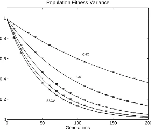
Fig. 1. Population fitness variance for five different selection schemes. Solid lines are analytical results and error bars are simulation results averaged over 10,000 runs. Curves presented are steady-state (SSGA), generation gap G=0.2, generation gap G=0.5, generational (GA), and a simple model of the CHC algorithm (CHC). Population size is 100.
Figure 1 shows a comparison of these analytical results with simulation data. A population of 100 was initially
drawn from a normal distribution (κ2 = 1) and selection
repeatedly performed. The plot shows the decreasing pop-ulation fitness variance for five different selection schemes — steady-state selection (SSGA), generation gapG= 0.2, generation gap G= 0.5, traditional generational selection (GA), and CHC style selection (CHC). Simulation data were averaged over 10,000 runs.
IV. Performing the Calculations
To calculateV[n] for each selection scheme is an exercise in probability. We use two results from standard probabil-ity theory regarding binomial and hypergeometric distri-butions [14].
Selecting from a population with replacement gives rise to a binomial distributionB(N, p) where we selectN times with probability of success p. In this case, the expected number of times any individual is selected and its variance are given by,
E[n] =Np V[n] =Np(1−p).
When we are selecting without replacement, the result is a
hypergeometric distribution H(M, m, N). Here M is the
size of the population,N is the number of times we select
and m is the number of copies of each individual in the
initial population. This gives the known result,
E[n] =Nm
M V[n] =
Nm(M −N) (M−m) M3−M2 .
In each case we calculateE[n] to check that population size is conserved, as expected, and then use V[n] in eqn. (11) to give the expected change in population fitness variance and thus the rate of genetic drift.
A. Generational Selection
In a generational selection scheme under random
sam-pling, we are drawingP members from a population with
replacement. This gives rise to a binomial distribution, B(P,1/P) and thus,
E[n] = 1
V[n] = 1−1/P.
As required E[n] = 1 and we can thus substitute V[n] directly into eqn. (11) to give,
E[κ2] =
1− 1
P
κ2. (13)
Using the definition ofrin eqn. (12),
r= 1− 1
P. (14)
B. Steady-State Selection
In the steady-state genetic algorithm we select one mem-ber at random, replicate it, and replace another random member with the copy in each time step.
We can calculate this by dividing the population into two. We draw one member with replacement into
subpop-ulation A and then drawP−1 members without
replace-ment into subpopulation B. We then combine these two to form the next population. For subpopulation A we have a binomial distributionB(1,1/P) and hence,
E[nA] = 1/P
V[nA] = (P−1)/P2.
For subpopulation B we have a hypergeometric distribution H(P,1, P −1) and hence,
E[nB] = 1−1/P
V[nB] = (P−1)/P2.
Since the two populations are independent, we can simply sum for the final population,
E[n] = E[nA] +E[nB] = 1
V[n] = V[nA] +V[nB] = 2(P−1)/P2.
As required E[n] = 1 and we can thus substitute V[n] directly into eqn. (11) to give,
E[κ2] =
1− 2
P2
κ2. (15)
the change after one generation,
r =
1− 2
P2
P
≈ 1− 2
P. (16)
It is clear that the rate of genetic drift is twice that of the generational case.
C. Varying Generation Gap
To generalise between these two cases we use the
con-cept of generation gap (G). We selectGP members with
replacement from the original population and delete GP
members at random to make room.
Again we can consider two subpopulations. We drawGP
members with replacement from the original population
into subpopulation A and then draw P(1−G) members
without replacement into subpopulation B.
For subpopulation A we have a binomial distribution B(GP,1/P) and hence,
E[nA] =G
V[nA] =G(1−1/P).
For subpopulation B we have a hypergeometric distribution H(P,1, P −GP) and hence,
E[nB] = 1−G
V[nB] =G−G2.
Again we simply sum these for the final population,
E[n] = 1
V[n] = 2G−G2−G/P.
As required E[n] = 1 and we can thus substitute V[n] directly into eqn. (11) to give,
E[κ2] =
1−2G−G
2−G/P
P−1
κ2. (17)
To compare this to one generation we apply the selection
operator 1/G times. Thus approximating to first-order
terms in 1/P we get,
r =
1−2G−G
2−G/P
P−1
1
G
≈ 1−2−G
P . (18)
Thus there is a gradual transition between the two rates of genetic drift as generation gap changes.
D. CHC Algorithm and Evolution Strategies
Eshelman’s CHC algorithm uses another non traditional form of selection whereby crossover is performed amongst
the initial population and then selection is performed with-out replacement from the combined population of parents and offspring.
A simple model of this used by Schaffer et al. [2] in
a numerical genetic drift comparison is to duplicate each
member of the population and then drawP members from
the population of 2P without replacement. In terms of
evolution strategies this is (μ+λ) selection withλ=μ. This selection gives rise to a hypergeometric distribution H(2P,2, P) where we selectP times from an initial popu-lation of 2Pwhich consists of two copies of each individual.
E[n] = 1
V[n] = (P−1)/(2P−1).
As required E[n] = 1 and we can thus substitute V[n] directly into eqn. (11) to give,
E[κ2] =
1− 1
2P−1
κ2. (19)
As we drawP members from the population, we can
com-pare this directly to the generational case and simply make a first-order approximation,
r≈1− 1
2P. (20)
Thus genetic drift in this model of CHC selection is at half the rate of that of the traditional generational algorithm.
Whilst we have only considered the case here equivalent to CHC selection, the technique presented is immediately applicable to other evolution strategy selection schemes.
When λ is a whole number multiple of μ, the above
ap-proach gives the correct expression. However the more
common and more interesting case whereλis some fraction
of μis more complicated due to the need to average over
the population.
We consider a (μ+λ) evolution strategy where μ= P
andλ=sP wheresis some fraction, 0≤s≤1. When we
apply selection, we are selecting from two subpopulations, one consisting ofP(1−s) individuals and the other of size 2sP containingsP pairs. Ifn1is the number of individuals
and n2 the number of pairs in the final population, the
variance in the number of times any population member is selected can be shown to be simply,
V[n] = 2n2
P , (21)
as PE[n] = n1+ 2n2, PEn2 =n1+ 4n2, E[n] = 1 and
V[n] =En2−E[n]2. If we drawXtimes without replace-ment from the subpopulation of pairs, the number of pairs drawn and thus the number of pairs in the final population is given by,
n2 = X 2−X
2 (2sP−1) (22)
Substituting eqn. (22) into eqn. (21) and averaging overX gives,
V[n] = E
X2−E[X]
The expectations of X are described by the hypergeomet-ric distribution H(P(1 +s),2sP, P), as we are drawingP times without replacement from a population ofP(1 +s). Using V[X] = EX2−E[X]2 and the standard results for the hypergeometric distribution given earlier, gives the result,
V[n] = 2s(P−1)
(1 +s) [P(1 +s)−1]. (24)
As before, we can substitute V[n] directly into eqn. (11) and normalise the expression by applying the selection 1/s times to give the final rate of genetic drift,
r =
1− 2s
(1 +s) [P(1 +s)−1]
1/s
≈ 1− 2
(1 +s)2P. (25)
The rate of genetic drift covers the same range as that seen for the genetic algorithm selection schemes. Figure 2 shows a plot of these analytical result against simulation
data. Four different values of s are considered and the
population size is again 100.
0 50 100 150 200
0 0.2 0.4 0.6 0.8 1
Generations
Population Fitness Variance
s=1
s=1/P
s=0.5
[image:5.595.83.283.212.267.2]s=0.2
Fig. 2. Population fitness variance for (μ+sμ) selection for varying s. Solid lines are analytical results and error bars are simulation results averaged over 10,000 runs. Popula-tion size is 100.
V. Discussion
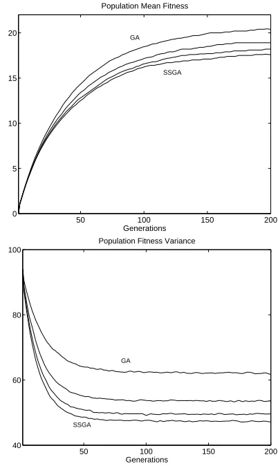
Analysing genetic drift in terms of the change in popula-tion fitness variance allows exact analytical expressions to be derived for any selection scheme. From these expressions we can make some comparisons of the effect that genetic drift has on the convergence of a GA under varying gener-ation gap. If we consider a GA using a small populgener-ation and weak selection, these effects will be most pronounced. Figure 3 shows the population fitness mean and variance for steady state, generational, and varying generation gap
(G = 0.2 and 0.5) implementations of GA on the
ONE-MAX problem. All use a population size of 50 with prob-abilistic tournament selection (s = 0.1), string length 96,
point mutation rate 1/96, and uniform crossover. CHC is
not included in the comparison as the other features of the algorithm lead to more significant differences than genetic drift alone.
Selection pressure is the same in each case as evidenced by the identical initial gradients of the mean fitness curves. As variance decreases through selection, the change in mean fitness decreases. For the steady state GA, variance decreases fastest due to the higher rate of genetic drift and thus the mean fitness evolves to a lower final value.
50 100 150 200
0 5 10 15 20
Population Mean Fitness
Generations GA
SSGA
50 100 150 200
40 60 80 100
Generations Population Fitness Variance
GA
[image:5.595.330.531.220.557.2]SSGA
Fig. 3. Population mean fitness and variance for four dif-ferent selection schemes. Simulation results are averaged over 10,000 runs and the error bars are the thickness of the lines. Curves presented are (in order) steady-state (SSGA), generation gap G=0.2, generation gap G=0.5, and genera-tional (GA).
[image:5.595.43.294.348.558.2]factor, alongside more commonly understood factors such as selection pressure, which affects the convergence of the GA and can be controlled by the choice of selection scheme.
Acknowledgments
The authors would like to thank the reviewers for high-lighting the use of the hypergeometric probability distri-bution and suggestions on notation. Both contridistri-butions improve the clarity of the calculations.
Alex Rogers is supported by an award from the EPSRC - Engineering and Physical Science Research Council.
References
[1] K. A. De Jong, An Analysis of the Behaviour of a Class of Genetic Adaptive Systems, Ph.D. thesis, University of Michigan, 1975.
[2] J. Schaffer, M. Mani, L. Eshelman, and K. Mathias, “The Ef-fect of Incest Prevention on Genetic Drift,” inFoundations of Genetic Algorithms 5, W. Banzhaf and C. Reeves, Eds., San Francisco, 1998, Morgan Kaufmann, In press.
[3] P. A. P. Moran, “Random Processes in Genetics,” Proceedings of the Cambridge Philosophical Society, vol. 54, pp. 60–71, 1958. [4] M. Kimura, Diffusion Models in Population Genetics, Ap-plied Probability. Methuen’s Review Series in ApAp-plied Proba-bility, 1964.
[5] W. J. Ewens, Mathematical Population Genetics, Springer-Verlag, 1979.
[6] A. Pr¨ugel-Bennett and J. L. Shapiro, “An Analysis of Genetic Algorithms Using Statistical Mechanics,” Phys. Rev. Lett., vol. 72, no. 9, pp. 1305–1309, 1994.
[7] A. Pr¨ugel-Bennett and J. L. Shapiro, “The Dynamics of a Ge-netic Algorithm for Simple Random Ising Systems,” Physica D, vol. 104, pp. 75–114, 1997.
[8] A. Pr¨ugel-Bennett, “Modelling Evolving Populations,”J. Theor. Biol., vol. 185, pp. 81–95, 1997.
[9] M. Rattray,Modelling the Dynamics of Genetic Algorithms us-ing Statistical Mechanics, Ph.D. thesis, Manchester University, Manchester, UK, 1996.
[10] H. M¨uhlenbein, “Genetic Algorithms,” inLocal Search in Com-binatorial Optimization, E. Aarts and J. K. Lenstra, Eds., New York, 1997, pp. 137–171, Jon Wiley and Sons.
[11] K. A. De Jong and J. Sarma, “Generation Gaps Revisited,” in
Foundations of Genetic Algorithms 2, L. Darrel Whitley, Ed., San Mateo, 1993, pp. 19–28, Morgan Kaufmann.
[12] L. Eshelman, “The CHC Adaptive Search Algorithm: How to Have Safe Search When Engaging in Nontraditional Genetic Re-combination,” inFoundations of Genetic Algorithms 1, G. Rawl-ins, Ed., San Mateo, 1991, pp. 265–283, Morgan Kaufmann. [13] A. Rogers and A. Pr¨ugel-Bennett, “Modelling the Dynamics of
Steady-State Genetic Algorithms,” in Foundations of Genetic Algorithms 5, W. Banzhaf and C. Reeves, Eds., San Francisco, 1998, Morgan Kaufmann, In press.