The Fast Parametric Integral Equations System for
Polygonal 2D Potential Problems
Andrzej Ku˙zelewski and Eugeniusz Zieniuk
Abstract—Application of techniques for modelling of bound-ary value problems implies three conflicting requirements: obtaining high accuracy of the results, high speed of the solution and low occupancy of computers memory (RAM). It is very difficult to satisfy such requirements particularly in process of solving large-scale engineering problems. Numerical solution of these problems require computations on large matrices. Accurate results can be obtained only by using appropriate models and algorithms. In the previous papers the authors applied the parametric integral equations system (PIES) in modelling and solving boundary value problems. The first requirement was satisfied - the results were obtained with very high accuracy. This paper fulfils other requirements by novel approach to accelerate the PIES. For this purpose the fast multipole method (FMM) is included into conventional PIES, therefore the fast PIES method is obtained.
Index Terms—parametric integral equations system, bound-ary value problems, fast multipole method.
I. INTRODUCTION
F
OR many years the authors of this paper have worked on development and application of the parametric integral equations system (PIES) to solve boundary value problems. The PIES has already been used to solve problems modelled by 2D and 3D partial differential equations, such as: Laplace [1], [2], Helmholtz [3] or Navier-Lam´e [4], [5], [6]. The remarkable advantage of the PIES, compared to traditional boundary integral equation (BIE), is direct inclusion in its mathematical formalism a shape of the boundary of the considered problem [7]. The shape of the boundary is gen-erally defined using particular functions. For this purpose, the curves (eg. B´ezier, B-spline, etc.) or surface patches (such as Coons, B´ezier and others) widely used in computer graphics, were applied in the PIES. The PIES is an analytical modification of traditional BIE. The above mentioned curves and surface patches are applied in modelling the shape of the boundary, instead of the contour integral as in the case of BIE. Therefore in practice, a small number of control points is required to define any shape of the boundary. It is definitely much easier than in case of element methods (such as boundary element method BEM [8] or finite element method FEM [9]). Moreover, the accuracy of solutions can be efficiently improved without interference in modelling the shape of the boundary.The former studies focused on accuracy and efficiency of the results obtained using the PIES in comparison with the well-known algorithms such as the FEM or the BEM, as well as analytical methods. These studies confirmed the effectiveness and accuracy of the PIES in solving 2D [1], [4] and 3D [2], [5], [7] boundary value problems. The authors
Manuscript received March 14, 2017; revised April 14, 2017.
A. Ku˙zelewski and E. Zieniuk are with the Faculty of Mathematics and Informatics, University of Bialystok, 15-245 Białystok, Ciołkowskiego 1M, Poland, e-mails: [email protected], [email protected].
also proposed some extensions of the PIES method, i.e. to solve uncertainly defined problems (interval PIES [10], [11]) or to solve transient problems [12]. The former studies show, that modelling of the boundary in the PIES is definitely more simple and efficient compared to the FEM or the BEM. However efficient solving of large-scale engineering problems by the PIES is limited (similarly to conventional BEM) due to the fact, that the PIES in general produces dense and non-symmetrical matrices. That matrices are definitely smaller in sizes than in the BEM, although to compute their coefficients we needO(N2)operations and anotherO(N3)
operations to solve obtained system using direct solvers (whereN - the number of equations of the algebraic system of linear equations).
In the paper [13] the authors proposed parallel version of the PIES obtained using OpenMP, while in [14], [15], [16] they accelerated numerical computing of coefficients and solving of the system of linear equations using CUDA [17]. These approaches reduce quite significantly the time of computations, however the problem of limited resources of RAM in PC still exists. Therefore, it not allows for convenient and efficient solving of large-scale engineering problems.
In the mid of 1980s of XX century Rokhlin and Greengard proposed the fast multipole method (FMM) [18], [19], [20], which allows to reduce the CPU time in the FMM accelerated methods toO(N), as well as definitely reduce occupancy of RAM. However, application of the FMM has increased the complexity of implementation of the PIES. It requires a new approach for computing coefficients and solving the system of linear equations.
The main goal of this paper is to present possibility of acceleration of the PIES for numerical solving of boundary value problems using the FMM. The main concept of the FMM is adopted from the FMM-BEM method [20]. However we think, that inclusion of the FMM into the PIES should be more effective than into the BEM. It is strictly connected with the different way of defining of BRC in the PIES and the BEM. To verify this concept, we need to include the FMM into conventional PIES. Additionally, we must modify the way of solving of the linear system of equations and apply iterative solver. Therefore, we obtain the new fast PIES method. In our preliminary studies we try to confirm high efficiency of the fast PIES on the example of polygonal 2D potential boundary problem.
II. THEPIESFOR TWO-DIMENSIONAL POTENTIAL BOUNDARY PROBLEM
using boundary integrals. The main goal of modification was inclusion of the shape of boundary in mathematical formalism of BIE. The shape of boundary is defined by parametrical linear (or non-linear) functions. The PIES for polygonal domains is presented by the following formula [7]:
1
2ul(sk) = n X
j=1
( sj
Z
sj−1
U∗lj(sk, s)pj(s)ds−
− sj
Z
sj−1
P∗lj(sk, s)uj(s) )
Jj, (1)
where: l = 1,2, ..., n, sl−1 ≤sk ≤sl, sj−1 ≤s≤sj, Jj is the Jacobian,nis the number of parametric segments that creates polygonal boundary of domain in 2D. In PIES defined in the parametric reference system,sl−1andsj−1correspond
to the beginning of l-th and j-th segment, while sl andsj to their ends.
Integrands U∗lj(sk, s)and P ∗
lj(sk, s) in (1) are presented in the following form:
U∗lj(sk, s) = 1 2πln
1
p
S12+S22 ,
P∗lj(sk, s) = 1 2π
S1n(1j)+S2n(2j) S2
1+S22 ,
(2)
where:S1=Sl(1)(sk)−Sj(1)(s)andS2=S
(2)
l (sk)−S(2)j (s). ExpressionsSn(i)(s) (n=j, l, i= 1,2)are parametric linear functions
Sn(i)(s) =a
(i)
n s+b
(i)
n , (3)
which describe particular segments of polygonal domain. Coefficients a(ni) and b(ni) are obtained in an easy way by simple algorithm utilizing corner points of polygon.
Similarly to the previous researches [1], [3], [6], the pseudospectral method [22] was applied to numerical solving of the PIES (1). Boundary functions are approximated by the following series:
uj(s) = N X
k=0
u(jk)L(jk)(s),
pj(s) = N X
k=0 p(jk)L
(k)
j (s),
(4)
where u(jk) and p(jk) are unknown coefficients on segment
j, N - is the number of terms in approximating series (4),L(jk)(s)- the base functions (Lagrange polynomials) on segmentj.
Finally, an algebraic version of PIES (1) is transformed into system of algebraic equationsAx=b. To solve the sys-tem, Gaussian elimination with partial pivoting and iterative refinement is used. Solutions on the boundary are obtained after solving the system.
III. THE FASTPIESFORMULATION
The FMM is applied to accelerate the solving of equation (1). The main idea of the FMM is to transform calculating interactions between segments into interactions between the cells that create the hierarchical structure (tree) with the
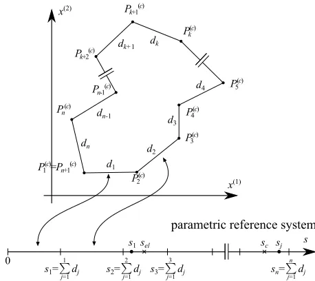
smallest cells (called leaves) containing a number of seg-ments. Because the PIES for 2D problems is defined on parametric line s (Fig. 1), the tree structure is created on the basis of that line, unlike in the FMM-BEM [21], where whole plane is used. Example of the tree structure for the fast PIES is presented in Fig. 2.
P2(c)
x(2)
x(1)
P1(c)=Pn+1(c)
P3(c)
P4(c)
P5(c)
Pk(c)
Pk+1(c)
Pn(c)
Pn-1(c)
Pk+2(c)
s d1
d2
d3
d4
dk
dk+1
dn-1
dn
0
s1= dj P
j=1 1
s2= dj P
j=1 2
s3= dj P
j=1 3
sn= dj P
j=1 n
parametric reference system
sel sc
[image:2.595.309.538.146.350.2]s1 sj
Fig. 1. Mapping of the shape of the boundary into parametric reference system
On the basis of the tree the following steps of the FMM procedure are performed: multipole expansion (calculation of moments), moment translation, moment-to-local translation and moment-to-local-to-moment-to-local translation. During the computations, the complex notation is introduced, due to convienient describing of points on the plane. They are reduced to the form ofP1(c)=P1(1)+iP1(2) (Fig. 1), where (c) - complex, (1) - coordinate in direction x(1), (2) -coordinate in directionx(2),i=√−1.
cell
leaf
Level
0
1
2
3
4
8 9 10 11 12 13 14 15
16 17 18 19
1
2 3
[image:2.595.316.540.531.694.2]4 5 6 7
Fig. 2. Example of the tree structure for the fast PIES
1) Multipole expansion: At first, we consider the integral
noted, that:
U∗lj(sk, s) =− 1 2πln
q
S2
1+S22=
=− 1 2πℜ
n
ln S
(c)
l −S
(c)
j o
=ℜnU∗lj(c)(sk, s) o
,
(5)
where Sl(c) = Sl(1) + iSl(2), Sj(c) = S
(1)
j +iS
(2)
j and
U∗lj(c)(sk, s) =−21πln S
(c)
l −S
(c)
j
,ℜ- real part of complex
number. The collocation pointsk is located in the segment
Sl(c), and observation pointsj in the segment S
(c)
j .
Assuming that introduced pointsc(located in the segment
Sc(c)), which is the key element of the FMM, is close to the pointsj(Fig. 1), the kernel can be expanded aboutS
(c)
c using the Taylor series expansion:
U∗lj(c)(sk,s) = 1 2π
(
−ln
S
(c)
l −S
(c)
c + + ∞ X k=1
(k−1)!
h
S(lc)−S
(c)
c ik
h
S−Sc(c) ik
k!
)
.
(6)
In order to simplify the calculations we should change the base of integrations into S similarly to (3):S =ajs+bj, where aj =
Pj(c)−Pj(c)
−1
dj−1 and bj = P
(c)
j−1−
(Pj(c)−Pj(c)
−1)sj−1
dj−1 ,
j= 1,2, ..., n. Therefore, new limits of integration arePj(−c)1
(lower) andPj(c)(upper). We also need to changedsbydS:
dS
ds =aj => ds= dS aj
.
Substituting the kernel U∗lj(c)(sk, s) into integral (1) and
Wj =aj, we obtain the following expression: sj
Z
sj−1
U∗lj(c)(sk, s)pj(s)ds=
= Pj(c) Z
Pj(c)
−1
1 2πpj(S)
(
−ln
S
(c)
l −S
(c)
c 1 Wj + + ∞ X k=1
(k−1)!
h
Sl(c)−Sc(c) ik
h
S−Sc(c) ik
k!·Wj ) dS= = 1 2π ∞ X k=0 Uk(S
(c)
l , S
(c)
c )Mk(Sc(c)),
(7)
whereMk(S( c)
c )are called moments aboutSc(c):
Mk(Sc(c)) = Pj(c) Z
Pj(c)
−1
h
S−Sc(c) ik
k!
pj(S)
Wj
dS.
They are independent of the collocation pointsk and should be computed once only. ExpressionsUk(S(
c)
l , S
(c)
c )have the following form:
Uk(S
(c)
l , S
(c)
c ) =
−ln
S
(c)
l −S
(c)
c
fork= 0
(k−1)!
S(c)l −S(c)c
k fork≥1
wheresc are mid-point of leaves.
2) Moment-to-moment translation: If we want to move
the pointsc to a new locations ′
c (when we change the level of the tree during computations), we can use the following expression to find new moments abouts′
c:
Mk(S
′(c)
c ) =
Pj(c) Z
Pj(c)
−1
h
S−Sc′(c) ik
k! ·
pj(S)
Wj
dS. (8)
Taking into account, that:
h
S−Sc′(c) ik
k! =
h
(S−Sc(c)) + (S( c)
c −S
′(c)
c )
ik
k! and applying the binomial formula:
(a+b)n = n X m=0 n m
ambn−m (9)
at last we obtain moments in the points′ c:
Mk(S
′(c)
c ) =
k X
m=0
h
S(cc)−S
′(c)
c
i(k−m)
(k−m)! Mm(S
(c)
c ) (10)
using a finite number of term in the translation.
3) Moment-to-local translation: Assuming, that the point
sel is close to the collocation point sk (see Fig. 1), the equation (7) can be expanded aboutSel(c)(the segment, where the pointsel is located) using the Taylor series expansion:
sj
Z
sj−1
U∗lj(c)(sk,s)pj(s)ds=
= 1
2π
∞ X
l=0 Ll(S
(c)
el , S
(c)
c )
h
Sl(c)−Sel(c)i
l
l!
(11)
where:
L0(Sl(c), S
(c)
c ) =−ln
S
(c)
el −S
(c)
c M0(S
(c)
c )+
+ ∞ X
k=1
(k−1)!·Mk(S( c)
c )
h
Sel(c)−Sc(c) ik
and
Ll(S
(c)
l , S
(c)
c ) = (−1) l
∞ X
k=0
(k+l−1)!·Mk(S
(c)
c )
h
Sel(c)−Sc(c)
ik+l forl≥1.
Pointssel, similarly tosc, are mid-points of leaves. Described procedure is also called local expansion.
4) Local-to-local translation: Similarly to
moment-to-moment translation, the point sel can be moved to new location s′
el (when we change the level of the tree during computations). It is performed using the binomial formula (9) and the following transformation:
∞ X l=0 l X m=0 = ∞ X m=0 ∞ X
l=m
At last we obtain the following local-to-local translation: sj
Z
sj−1
U∗lj(c)(sk, s)pj(s)ds= 1 2π
∞ X
l=0
(−1)l ·
·
( ∞
X
k=0
∞ X
m=l
(k+m−1)!·Mk(S( c)
c )
h
Sel(c)−Sc(c)
ik+m ·
· h
S′(c)
el −S
(c)
el im−l
(m−l)!
)
· h
Sl(c)−S′(c) el
il
l! .
(12)
5) Translations for the kernel P∗lj(sk, s): The kernel
P∗lj(sk, s)in the complex notation can be computed on the basis of the following expression:
P∗lj(c)(sk, s) =
∂U∗lj(c)(sk, s)
∂n(c) =n (c)∂U
∗(c)
lj (sk, s)
∂S , (13)
wheren(c)=n1+in2- normal vector to segmentj in the
complex notation. Hence
P∗lj(sk, s) =ℜ n
P∗lj(c)(sk, s) o
=
n1ℜ
∂U∗lj(c)(sk, s)
∂S
−n2ℑ
∂U∗lj(c)(sk, s)
∂S
,
(14)
whereℜ,ℑ- real and imagine part of complex number. Finally, after calculating the derivative (13) we obtain:
sj
Z
sj−1
P∗lj(c)(sk, s)uj(s)ds=
= 1
2π
∞ X
k=1 Pk(S(
c)
l , S
(c)
c )Nk(Sc(c)), (15)
where
Nk(Sc(c)) = Pj(c) Z
Pj(c)
−1
h
S−Sc(c) ik−1
(k−1)!
uj(S)n(c)
Wj
dS.
ExpressionsNk(S( c)
c ), similarly toMk(S( c)
c )(7), are called moments aboutSc(c)and they are independent of the colloca-tion pointskand should be computed once only. Expressions
Pk(Sl(c), Sc(c))have the following form:
Pk(S
(c)
l , S
(c)
c ) =
(k−1)!
h
Sl(c)−Sc(c)
ik for k≥1,
wheresc are mid-point of leaves.
It can be noted, that all translations described in pre-vious subsections remain exactly the same for the kernel
P∗lj(c)(sk, s), except for the fact that N0(S
(c)
c ). Therefore,
we can directly applied them for the momentsNk(S( c)
c ).
6) The fast PIES algorithm: The fast PIES algorithm runs
in several steps. The first step is to determine the structure of the tree. On the basis of 2D problems mapped into parametric reference system (Fig. 1) the structure of the tree is created. Level 0 cell covers the whole problem. It is the straight line where the PIES is defined. The length of this line is equal to
the sum of all segments, which created the boundary of the problem. Level 0 parent cell is divided into two equal child cells of level 1. Then, dividing is continued in the same way for each level parent cells. The division is carried out until the number of segments in a cell is less than or equal to the predefined maximum number of segments in a cell. Each cell, which has no children, is called a leaf. The division is completed if at the highest level we obtained leaves only or predefined maximum number of levels is reached.
The next step is called upward pass. Starting from the highest number level, moments in all leaves are computed (up tokterms in the Taylor series expansion). Then, tracing the tree structure upward and using moment-to-moment translation, all moments are computed in each parent cell, up to the level 2 (Fig. 3).
s1
s''el sc
s'el
sc s'el
s''c
moment-to-moment translations
sel
s''el
s'c s'c
local-to-local translations
moment-to-local translation
Level
2
3
4 1 0
[image:4.595.309.538.252.373.2]local expansion
Fig. 3. Translations in the fast PIES
The next step is called downward pass. To clearly de-scribed this pass, we should define a few terms connected with cells neighbourhood. Two cells are adjacent at leveliif they have common end. Two cells are well separated at level
iif they are not adjacent at leveli, but their parent cells are adjacent (at leveli−1). Then the interaction list of cell K
is created using the list of well-separated cells from a level
icellK. Two cells are far cells if their parent cells are not adjacent.
Coefficients of local expansion are computed starting from the level 2 and tracing the tree structure downward to all leaves (Fig. 3). Coefficients of local expansion at cell
K are the sum of the contributions from the cells in the interaction list of cell K (computed using moment-to-local translation) and from all the far cells (computed using local-to-local translation). For a cellKat level 2, only moment-to-local translation is used to compute coefficients of the moment-to-local expansion. At the highest number level, contributions from leafKand its adjacent cells are computed directly, as in the conventional PIES. Finally, we obtain a vector, which is the result of multiplication matrixAby a vectorxand there is no need to store the entire matrixAin the computer’s memory. This approach requires the use of iterative solvers for system of equations (eg. GMRES).
IV. TESTING EXAMPLE
with -O2 optimization. Numerical tests were carried out on 64-bit Ubuntu Linux operation system (kernel 4.4.0).
The testing example concerns the problem described by Laplaces equation. The shape of the boundary is shown in Fig. 4. It is simple boundary problem, however in order to increase its complexity, we assumed that the edge looks like a gear with 256 teeth. We used 512 linear segments to model the problem using both version of the PIES. Boundary conditions are identical on each tooth and they are presented in Fig. 4 (where p Neumanns and u Dirichlets boundary conditions). On each segment we have defined the same number of collocation points (from 2 to 8) and finally have solved the system of 1024 to 4096 algebraic equations. We assumed value of GMRES convergence criterion (GMRES tolerance) equal to 1e-8 and the number of terms in Taylor series is 15.
105 mm 100 mm
[image:5.595.332.516.240.379.2]u=10 p=1
Fig. 4. The shape of modelled problem
TABLE I
THE FASTPIESVS CONVENTIONALPIES: CPUTIME ANDRAM
OCCUPANCY
No. of CPU time [s]
Speed-up RAM occupancy [MB] equations fast PIES PIES fast PIES PIES
1024 0.31 3.06 9.87 1 37
2048 1.18 15.16 12.85 3 112
3072 2.11 43.49 20.61 7 228
[image:5.595.116.219.256.490.2]4096 3.58 94.28 26.34 12 396
Table I presents obtained results of accelerating calcu-lations in the fast PIES compared to conventional PIES. Growing number of equations results in small increase of computation time in the fast PIES, contrary to conventional PIES. The fast PIES also needs more than 30 times less RAM during computations.
Relative error normL2 between solutions obtained by the fast and conventional PIES is presented in Table II. The value ofL2for GMRES tolerance equal 1e-8 do not exceed 0.001% in all cases. Decreasing tolerance to 1e-6 results in grow of solutions errors (in the worst case L2 norm is less
TABLE II
ACCURACY OF THE FASTPIESSOLUTIONS VS VALUE OFGMRES
CONVERGENCE CRITERION
No. No. of iterations CPU time [s] Rel. error norm [%] of for GMRES tol. for GMRES tol. for GMRES tol. eq. 1e-8 1e-6 1e-8 1e-6 1e-8 1e-6 1024 38 9 0.31 0.25 8.36e-5 8.42e-4 2048 150 114 1.18 0.95 9.14e-4 9.26e-4 3072 184 144 2.11 1.72 6.82e-5 0.031 4096 291 176 3.58 2.61 2.41e-4 0.048
than 0.05%), however the number of iterations is reduced, as well as computation time.
0 500 1000 1500 2000 2500 3000 3500 4000 4500
0 10 20 30 40 50 60 70 80 90 100
Number of equations
CPU time [s]
conventional PIES fast PIES
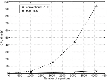
Fig. 5. Comparison of the CPU time used by the fast PIES and conventional PIES
Fig.5 presents comparison of used CPU time between conventional PIES and fast PIES. It should be noted, that the shape of plotted lines is consistent with theoretical considerations. Conventional PIES needsO(N2)operations
to compute their coefficients and anotherO(N3)operations
to solve the system by the direct solver. Application of the fast PIES is definitely more efficient.
Additionally, we solve the example using a bit old appli-cation of the FMM-BEM, which has been written in fortran by the authors of [21]. We want to find solutions comparable with the fast PIES, therefore the mesh in the FMM-BEM is composed of 1024, 2048, 3072 or 4096 linear elements (each teeth is describe by 4, 8, 12 or 16 elements). The example of discretization (for 1024 elements mesh) of a few teeth of the gear is presented in Fig. 6. Tolerance of GMRES is 1e-8 and the number of terms in Taylor series is 15.
TABLE III
THE FASTPIESVS THEFMM-BEM: CPUTIME ANDRAMOCCUPANCY
No. of CPU time [s] RAM occupancy [MB] equations fast PIES FMM-BEM fast PIES FMM-BEM
1024 0.31 0.78 1 5
2048 1.18 5.01 3 11
3072 2.11 24.17 7 18
4096 3.58 52.12 12 25
[image:5.595.311.543.653.728.2]u=10 p=1
[image:6.595.104.233.56.195.2]boundary element
Fig. 6. Example of the FMM-BEM discretization for 1024 elements mesh
the problem of the FMM-BEM is rather connected with too big size of allocated RAM compared to really used. Therefore, we can use maximum 70 elements in a cell.
0 1000 2000 3000 4000 5000
0 10 20 30 40 50 60
Number of equations
CPU time [s]
[image:6.595.76.263.288.386.2]FMM−BEM fast PIES
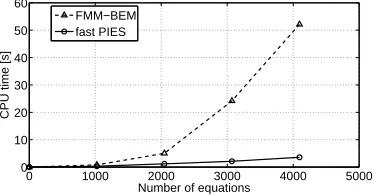
Fig. 7. Comparison of the CPU time used by the fast PIES and the FMM-BEM
Fig.7 presents comparison of used CPU time between the fast PIES and the FMM-BEM. Application of the fast PIES is more efficient than the FMM-BEM. However, we should highlight the fact, that the FMM-BEM program is a bit old. Additionally, relative error normL2 computed between the FMM-BEM and the fast PIES is smaller than 0.1%.
V. CONCLUSION
The paper presents possibility of acceleration of computa-tion and reduccomputa-tion RAM occupancy for numerical solving of boundary value problems using the PIES. Verification of this concept required inclusion of the FMM into conventional PIES. The numerical example shows significant reduction of computation time of the fast PIES. The speed-up in comparison to conventional PIES increases with the size of the considered problem. We noted almost no difference between accuracy of solutions obtained by the fast PIES and conventional one. The fast PIES is also slightly faster than the FMM-BEM, while accuracy of obtained results is almost the same.
This paper is our first attempt to use the fast PIES for solving 2D potential boundary value problems. The presented technique of acceleration of computations should be extended to the problems modelled by non-linear segments. Obtained results suggest that chosen direction of studies should be continued.
ACKNOWLEDGMENT
The authors would like to thank prof. Naoshi Nishimura from Department of Applied Analysis and Complex
Dynam-ical Systems Graduate School of Informatics, Kyoto Univer-sity, for sharing source code of the FMM-BEM application.
REFERENCES
[1] E. Zieniuk, “Modelling and effective modification of smooth boundary geometry in boundary problems using B-spline curves,”Engineering with Computers, Vol. 23, No. 1, pp. 39-48, 2007.
[2] E. Zieniuk and K. Szersze´n, “Triangular B´ezier surface patches in modelling shape of boundary geometry for potential problems in 3D,”
Engineering with Computers, Vol. 29, No. 4, pp. 517-527, 2013. [3] E. Zieniuk and K. Szersze´n, “Triangular B´ezier patches in modelling
smooth boundary surface in exterior Helmholtz problems solved by PIES,”Archives of Acoustics, Vol. 34, No. 1, pp. 51-61, 2009. [4] E. Zieniuk and A. Bołtu´c, “Non-element method of solving 2D
boundary problems defined on polygonal domains modeled by Navier equation,”International Journal of Solids and Structures, Vol. 43, No. 25-26, pp. 7939-7958, 2006.
[5] E. Zieniuk, A. Bołtu´c and K. Szersze´n, “Modeling complex homo-geneous regions using surface patches and reliability verification for Navier-Lam´e boundary problems,”Proceedings of The 2012 Interna-tional Conference on Scientific Computing WORLDCOMP 2012, pp. 166-172, 2012.
[6] E. Zieniuk, A. Bołtu´c and A. Ku˙zelewski, “Algorithms of identification of multi-connected boundary geometry and material parameters in problems described by Navier-Lam´e equation using the PIES,” in
Advances in Information Processing and Protection: International Advanced Computer Systems Conference 2006, pp. 409-418, 2006. [7] E. Zieniuk, “Computational method PIES for solving boundary value
problems (in polish),”PWN, Warszawa, 2013.
[8] C. A. Brebbia, J. C. F. Telles and L. C. Wrobel, “Boundary element techniques, theory and applications in engineering,”Springer-Verlag, New York, 1984.
[9] O. C. Zienkiewicz “The Finite Element Methods,” McGraw-Hill, London, 1977.
[10] E. Zieniuk and M. Kapturczak and A. Ku˙zelewski, “Concept of mod-eling uncertainly defined shape of the boundary in two-dimensional boundary value problems and verification of its reliability,” Applied Mathematical Modelling, Vol. 40, No. 23-24, pp. 10274-10285, 2016. [11] E. Zieniuk, A. Ku˙zelewski and M. Kapturczak, “The influence of interval arithmetic on the shape of uncertainly defined domains modelled by closed curves,”Computational & Applied Mathematics, doi:10.1007/s40314-016-0382-0, to be published.
[12] E. Zieniuk, D. Sawicki and A. Bołtu´c, “Parametric integral equations systems in 2D transient heat conduction analysis,”International Jour-nal of Heat and Mass Transfer, Vol. 78, pp. 571-587, 2014. [13] A. Ku˙zelewski and E. Zieniuk, “OpenMP for 3D potential boundary
value problems solved by PIES,”AIP Conference Proceedings 2016: 13th International Conference of Numerical Analysis and Applied Mathematics ICNAAM 2015, No. 480098, 2015.
[14] A. Ku˙zelewski and E. Zieniuk, “GPU-based acceleration of computa-tions in elasticity problems solving by parametric integral equacomputa-tions system,”Advances in Engineering Software, Vol. 79, pp. 27-35, 2015. [15] A. Ku˙zelewski, E. Zieniuk and M. Kapturczak, “Acceleration of integration in parametric integral equations system using CUDA,”
Computers & Structures, Vol. 152, pp. 113-124, 2015.
[16] A. Ku˙zelewski, E. Zieniuk and A. Bołtu´c, “Application of CUDA for Acceleration of Calculations in Boundary Value Problems Solving Using PIES,”,Lecture Notes in Computer Science: Parallel Processing and Applied Mathematics PPAM 2013, PT II, pp. 322-331, 2014. [17] “CUDA C Programming Guide,”
http://docs.nvidia.com/cuda/cuda-c-programming-guide/[access date: 03 March 2017].
[18] V. Rokhlin, “Rapid solution of integral equations of classical potential theory,”Journal of Computational Physics, Vol. 60, No. 2, pp. 187-207, 1985.
[19] L. F. Greengard and V. Rokhlin, “A fast algorithm for particle simulations,” Journal of Computational Physics, Vol. 73, No. 2, pp. 325-348, 1987.
[20] L. F. Greengard, “The rapid evaluation of potential fields in particle systems,”The MIT Press, Cambridge, 1988.
[21] Y. J. Liu and N. Nishimura, “The fast multipole boundary element method for potential problems: A tutorial,”Engineering Analysis with Boundary Elements, Vol. 30, No. 5, pp. 371-381, 2006.