Optimal finite precision controller realization of sampled data systems

(1)

On: 13 September 2007

Access Details: [subscription number 773565843] Publisher: Taylor & Francis

Informa Ltd Registered in England and Wales Registered Number: 1072954 Registered office: Mortimer House, 37-41 Mortimer Street, London W1T 3JH, UK

International Journal of Systems

Science

Publication details, including instructions for authors and subscription information: http://www.informaworld.com/smpp/title~content=t713697751

Optimal finite-precision controller realization of

sampled-data systems

R. H. Istepanian; S. Chen; J. F. Whidborne Online Publication Date: 01 April 2000

To cite this Article: Istepanian, R. H., Chen, S. and Whidborne, J. F. (2000) 'Optimal finite-precision controller realization of sampled-data systems', International Journal of Systems Science, 31:4, 429 - 438

To link to this article: DOI: 10.1080/002077200291019 URL:http://dx.doi.org/10.1080/002077200291019

PLEASE SCROLL DOWN FOR ARTICLE

Full terms and conditions of use:http://www.informaworld.com/terms-and-conditions-of-access.pdf

This article maybe used for research, teaching and private study purposes. Any substantial or systematic reproduction, re-distribution, re-selling, loan or sub-licensing, systematic supply or distribution in any form to anyone is expressly forbidden.

(2)

Downloaded By: [University of Southampton] At: 17:39 13 September 2007

International Journal of Systems Science, 2000, volume 31, number 4, pages 429± 438

Optimal ® nite-precision controller realization of sampled-data

systems

R

.

H

.

I

STEPANIAN

{

,

S

.

C

HEN

{

,

J

.

W

U

}

and

J

.

F

.

W

HIDBORNE

}

W e investigate the sensitivity of closed-loop stability with respect to® nite word length (FW L) e ects in the implementation of digital controller coe cients. The optimal realization of digital controller structures with® nite precision consideration is formu-lated as the solution of a constrained nonlinear optimization problem. A sophisticated optimization strategy involving the adaptive simulated annealing (ASA) optimizer is developed to provide an e cient computational method for searching the optimal FW L controller realization with maximum stability bound and minimum bit length require-ment. A numerical simulation example is presented to illustrate the e ectiveness of the proposed strategy.

1. Introduction

The recent advances in advanced control design methods means that there is a need for the e cient and accurate implementation of controllers with a

higher order than traditional PID controllers.

Although the number of controller implementations using ¯ oating-point processors is increasing due to their reduced price, for reasons of cost, simplicity, speed, memory space and ease-of-programming, the use of ® xed-point processors is more desirable for many industrial and consumer applications, particularly for mass market applications in the automotive and consumer electronics sectors. Thus, the consideration of FWL e ects is an important issue in modern indus-trial digital control applications.

The FWL e ects in digital signal processing have been extensively studied over the last two decades (Roberts and Mullis 1987). More recent studies have addressed

the FWL e ects and parameterization issues on digital controller realizations and relevant applications (Gevers

and Li 1993, Madievski et al. 1995, Istepanian et al.

1996, 1998 b, Istepanian 1997). However, few studies to date address the closed-loop stability issues and the relevant e ects of the ® nite-precision controller

realiza-tions (Moroneyet al. 1980, Fialho and Georgiou 1994).

For such systems, the formulation of a ® nite-precision controller structure with a too small word length may result in the loss of closed-loop system stability due to the well-known FWL e ects. This is an interesting prob-lem within the FWL parameterization framework that has not been studied extensively.

An earlier FWL stability measure, from which a mini-mum bit length that guarantees the closed-loop stability can be estimated for a digital controller realization, was

proposed by Moroney et al. (1980). However,

com-puting this measure explicitly seems numerically very di cult and is still an unsolved open problem. Recently, a tractable FWL stability measure, which is a lower bound of the stability measure given by

Moroneyet al. (1980), has been derived and design

pro-cedures that guarantee the stability of the resulting optimal FWL controller have been developed (Li 1998). An enhanced tractable FWL stability measure, which provides a better lower bound than the one

given by Li (1998), has been introduced (Istepanian et

al. 1998 a). Based on this enhanced lower bound of the

stability measure, an e cient optimization procedure has been formulated to derive the optimal PID

International Journal of Systems ScienceISSN 0020± 7721 print/ISSN 1464± 5319 online#2000 Taylor & Francis Ltd http://www.tandf.co.uk/journals/tf/00207721.html

Received 14 September 1998. Revised 12 April 1999.

{Department of Electrical and Computer Engineering, Ryerson Polytechnic University, 350 Victoria Street, Toronto, Ontario, Canada, M5B 2K3; e-mail: [email protected]

{Department of Electronics and Computer Science, University of Southampton, High® eld, Southampton SO17 1BJ, UK.

}National Key Laboratory of Industrial Control Technology, Institute of Industrial Process Control, Zhejiang University, Hangzhou, 310027 , People’s Republic of China.

(3)

controller realization with maximum stability bound

and minimum bit length (Chenet al. 2000) .

In this paper, we extend the framework presented by Chenet al. (2000) and re® ne the theoretical concepts to generalize its applicability to any digital controller struc-tures for sampled-data control systems. The problem is formulated as a constrained nonlinear optimization problem. As the cost function is smooth and non-convex, an e cient global optimization strategy based on the ASA (Ingber and Rosen 1992, Ingber 1996,

Rosen 1997, Chen et al. 1998) is developed to search

for the optimal FWL controller realization. The paper is organized as follows. In section 2, we present the problem formulation and establish notations and de® ni-tions of FWL stability measures. In section 3, we apply the results of section 2 to formulate the optimization framework for obtaining the optimal FWL controller realizations with maximum stability bounds and mini-mum bit length requirements. The detailed optimization procedure is presented in section 4, and a numerical ex-ample is given in section 5 to illustrate the e ectiveness of the proposed approach. The paper ends with conclu-sions in section 6.

2. FWL stability measures

In this section, we introduce the FWL stability

measures derived by Moroney et al. (1980), Li (1998),

Istepanianet al. (1998 a), and present some re® nements,

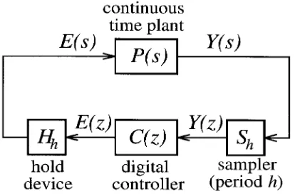
which will provide the basis for the derivation of the optimal FWL controller realization. Consider the sampled-data control system shown in ® gure 1, where

P…s†is the continuous-time linear time-invariant plant,

C…z†is the discrete-time linear shift-invariant controller,

Sh is the sampler with sampling periodh, andHh is the

hold device. The outputs of the sampler and hold device are given by

Y…z† ˆShY…s†: y…k† ˆy…t†jtˆkh …1†

and

E…s† ˆHhE…z†: e…t† ˆe…k†;kh<tµ …k‡1†h; …2†

respectively. Assume that P…s† is strictly proper. Let

…Ap;Bp;Cp;0†be a state-space description of P…s†, that

is, P…s† ˆCp…sI¡Ap†¡1Bp, where Ap2 Rm£m,

Bp2 Rm£l and Cp2 Rq£m. Let …Ac;Bc;Cc;Dc† be a

state-space description of C…z†, that is,

C…z† ˆCc…zI¡Ac†¡1Bc‡Dc, where Ac2 Rn£n,

Bc2 Rn£q, Cc2 Rl£n and Dc2 Rl£q. We will refer to

…Ac;Bc;Cc;Dc†as a realization of C…z†. The realizations

of C…z† are not unique. In fact, if …Ac;Bc;Cc;Dc† is a

realization of C…z†, so is …T¡1_A

cT;T¡1Bc;CcT;Dc†for

any similarity transformation_{T 2 R}n£n_.

Considering the behaviour of the sampled-data system at its sampling instants, we obtain a discrete-time feedback system:

Y…z† ˆShP…s†HhE…z†

E…z† ˆC…z†Y…z† 9 =

;: …3†

The plant P…z† ˆShP…s†Hh is the discretized P…s†, and

P…z† ˆCz…zI¡Az†¡1Bz has a state-space description

…Az;Bz;Cz;0†, where

AzˆeAph2 Rm£m;

Bzˆ

…h

0e

A_p½_B

pd½ 2 Rm£l and CzˆCp2 Rq£m: …4†

It can easily be seen that the corresponding state-space

description _…A-;B-;C-;D-†of the discrete-time closed-loop

system is given by:

-Aˆ

Az‡BzDcCz BzCc

BcCz Ac

2 4

3 5_ˆ Az

0

0 0

2 4

3 5_‡ Bz

0

0 In

2 4

3 5

£

Dc Cc

Bc Ac

2 4

3

5 Cz 0

0 In

2 4

3 5

ˆM0‡M1XM2ˆA-…X†; …5†

-Bˆ

Bz

0

2 4

3

5; C-ˆ ‰Cz 0Š; D-ˆ0; …6†

where M02 R…m‡n†£…m‡n†, M12 R…m‡n†£…l‡n† and

M2 2 R…q‡n†£…m‡n† are some ® xed matrices that

depend on P…s† and h, In denotes the n£n identity

[image:3.547.40.247.40.176.2]

matrix, and

(4)

Xˆ Dc Cc

Bc Ac

" #

ˆ

p1 p2 . . . pq‡n

pq‡n‡1 pq‡n‡2 . . . p2…q‡n†

.. .

. . . ... p_…l‡n¡1†…q‡n†‡1 p…l‡n¡1†…q‡n†‡2 . . . p…l‡n†…q‡n† 2 6 6 6 6 6 6 4 3 7 7 7 7 7 7 5

…7†

will be referred to as the controller matrix.

Suppose that C…z† has been given to make the

sampled-data system stable and the realization of C…z†

isX. Since the sampled-data system is stable if and only

if the system (3) is stable (Chen and Francis 1991), it

follows that the eigenvalues of A-…X†, denoted by

f¶i;1µiµm‡ng, satisfy j¶ij<1, 8i2 f1;. . .;m‡

ng. When the realization …Ac;Bc;Cc;Dc† of C…z† is

implemented in ® nite-precision format, the controller

matrixXis perturbed toX‡

D

X, where

D

Xˆ

D

p1

D

p2 . . .

D

pq‡n

D

pq‡n‡1

D

pq‡n‡2 . . .

D

p2…q‡n†

.. .

. . . ...

D

p…l‡n¡1†…q‡n†‡1

D

p…l‡n¡1†…q‡n†‡2 . . .

D

pN

2 6 6 6 6 6 6 6 6 4 3 7 7 7 7 7 7 7 7 5

…8†

and Nˆ …l‡n†…q‡n†. Due to the FWL e ects, each

element of

D

Xis bounded, that is,

·…

D

X†= max

i2f1;...;Ngj

D

pij µ

°

2: …9†

For a ® xed-point processor of Bs bits

°ˆ2¡…B_s¡B_X†_; _…₁₀_†

where BX is an integer and 2BX is a `normalization’

factor such that the absolute value of each element of

2¡B_X_X_{is not larger than 1. With the perturbation}

D

_X_,

¶iis moved to ¶~i. The closed-loop system is unstable if

and only if there exists i2 f1;. . .;m‡ng such that

j¶~ij ¶1.

To see when the round-o error will cause the

closed-loop system to become unstable, Moroney et al. (1980)

de® ned an FWL stability measure as:

·0…X†= inff·…

D

X†:A-…X† ‡M1

D

XM2 is unstableg:

…11†

How `robust’ a controller realization is to the FWL e ects can also be viewed from a di erent angle. Let

Bmins be the smallest word length that can guarantee

the closed-loop stability. It would be highly desirable

to know Bmin

s for a given controller realization.

However, except in simulation, it is impractical to test

the closed-loop system by reducingBs until it becomes

unstable. Based on ·0…X†, an estimate of Bmins is given

by

^

Bmins0 ˆInt‰¡log2…·0…X†Š ¡1‡BX; …12†

where Int_‰xŠ rounds x to the nearest integer and

Int_‰xŠ ¶x. From (9) to (12), we know that the

sampled-data closed-loop system is stable when X is

implemented with a ® xed-point processor of at least

^

Bmins0 bits. The problem with this FWL stability measure

is that computing explicitly the value of ·0…X†is still an

unsolved open problem. Thus, the stability measure

·0…X†has very limited practical value.

To overcome the di culty in the computation of

·0…X†, Istepanian et al. (1998 a) introduced an FWL

stability measure as:

·1…X†= min

i2f1;...;m‡ng

1_{¡ j}¶ij

XN jˆ1

@¶i

@pj X :

…13†

We have the following proposition.

Proposition 1: A-…X‡

D

X†is stable if·…

D

X†< ·1…X†.

Proof: When

D

Xis small, using a ® rst-order

approx-imation we assume

D

¶iˆ¶~i¡¶iˆ

XN jˆ1

@¶i

@p_{j X}

D

pj; 1µiµm‡n; …14†

where_¶~_i _{are the eigenvalues of} _A-_…_X_‡

D

_X_†_{. It follows}

that

j

D

¶ij µ

XN jˆ1

@¶i

@p_{j X}j

D

pjj µ·…

D

X†

XN jˆ1

@¶i

@p_{j X} : …15†

Thus, for 1µiµm‡n, if

·…

D

X†< 1¡ j¶ij

PN jˆ1 @¶_@_pi

j X ;

…16†

we have

j¶~ij µ j¶ij ‡ j

D

¶ij µ j¶ij ‡·…

D

X†

XN jˆ1

@¶i

@p_{j X}

<j¶ij ‡ 1¡ j¶ij

XN jˆ1

@¶i

@p_{j X}

XN jˆ1

@¶i

@p_{j X} ˆ1;…17†

which means thatA-…X‡

D

X†is stable. &

(5)

The assumption that the controller coe cient perturbations are very small is generally valid. For example, standard ® xed-point processors have 16 bits.

Assuming BXˆ4, then the controller parameter errors

are bounded by 2¡13_{. Notice that}

·1…X† is a lower

bound of ·0…X†. The proof is straightforward. De® ne

the set

PX= f

D

X:A-…X‡

D

X†is unstableg: …18†

For any

D

X2 PX, we must have ·1…X† µ·…

D

X†;

otherwise, according to Proposition 1, A-…X‡

D

X† is

stable, which is a contradiction. By the de® nition of

·0…X†, it follows that·1…X† µ·0…X†.

Unlike·0…X†,·1…X†is a tractable stability measure as

it can be computed easily using the following lemma.

The proof of this lemma is given by Istepanian et al.

(1998 a).

Lemma 1: L etA-…X† ˆM0‡M1XM2be diagonalizable and have f¶i;iˆ1;. . .;m‡ng as its eigenvalues, andxi

be a right eigenvector ofA-…X†corresponding to the

eigen-value ¶i. Denote Mxˆ ‰x1¢ ¢ ¢xm‡nŠ and Myˆ

‰y1¢ ¢ ¢ym‡nŠ ˆMx¡H, where yi is called the reciprocal

left eigenvector corresponding to ¶i, and H denotes the

transpose and conjugate operation. Then

8i2 f1;. . .;m‡ng

@¶i

@Xˆ

@¶i

@p1

@¶i

@p2 . . .

@¶i

@pq‡n

@¶i

@pq‡n‡1

@¶i

@pq‡n‡2 . . .

@¶i

@p2…q‡n†

.. . .. . . . . ... @¶i

@p_…l‡n¡1†…q‡n†‡1

@¶i

@p_…l‡n¡1†…q‡n†‡2 . . .

@¶i

@pN

2 6 6 6 6 6 6 6 6 6 6 6 6 6 6 6 4 3 7 7 7 7 7 7 7 7 7 7 7 7 7 7 7 5

ˆM1Ty¤ixTiM2T; …19†

where T denotes the transpose operation, and ¤ _the con-jugate operation.

When a designed in® nite-precision stable controllerX

is implemented with a ® xed-point processor of Bs bits,

the norm of the controller perturbation·…

D

X†and the

lower-bound stability measure ·1…X† can be evaluated.

According to Proposition 1, if ·1…X†> ·…

D

X†, the

closed-loop stability is maintained. Furthermore, from (9) and (10), it is easily seen that the closed-loop system

is stable if ·1…X†>…2¡…Bs¡BX††=2. De® ne

^

Bmins1 ˆInt‰¡log2…·1…X†Š ¡1‡BX: …20†

It can be used as an estimate of Bmins . Obviously, as

^

Bmins1 ¶B

^

mins0 ¶Bmins , B

^

mins1 is a more conservative

estimate ofBmin

s thanB

^

mins0 . However,B

^

mins0 is impractical

to obtain.

Another tractable FWL stability measure, introduced by Li (1998), is de® ned as

·2…X†= min

i2f1;...;m‡ng

1¡ j¶ij

NX

N jˆ1

@¶i

@p_{j X}

2 v

u u

t _:

…21†

It is also a lower bound of ·0…X†. Similarly, an

estimate _B

^

min

s2 of Bmins can be computed based on

·2…X†. Since

XN jˆ1

@¶i

@p_{j X}

…

†

2µNX

N jˆ1

@¶i

@p_{j X}

2

; …22†

where the equality only holds under a very restricted

condition, we have ·2…X† µ·1…X† µ·0…X†. It follows

that_B

^

min

s2 ¶B

^

mins1 . Thus,·1…X†, which is closer to·0…X†,

is a better FWL stability measure and can provide a

better estimate of Bmin

s .

3. Optimal FWL controller realization

Since·1…X†is a better tractable FWL stability measure

than·2…X†, we will use it as the basis for the derivation

of the optimal FWL controller realization problem. It is

known that there are di erent realizationsXfor a given

C…z†, and the stability measure·1…X†is a function of the

realization. It is of practical importance to ® nd a

realiza-tion that maximizes·1…X†. Such a realization is optimal

in the sense that it has maximum closed-loop stability robustness to FWL e ects. The digital controller imple-mented with an optimal realization can guarantee the stability of the closed-loop system with a minimum hardware requirement in terms of word length.

To start the optimal design procedure, it is assumed

that an initial realization of C…z†,

X0ˆ D0

c C0c

B0c A0c

2 4

3

5; …23†

is available. Any realization ofC…z†can be expressed as:

X_T = Il 0

0 _T¡1

2 4

3 5X0

Iq 0

0 _T

2 4

3

5; …24†

where_{T 2 R}n£n _{and det}

…T † 6ˆ0. From (5), the

(6)

-A…X_T† ˆ Az

0

0 0

" #

‡ Bz

0

0 In

" # _I

l 0

0 _T¡1

" #

X0 Iq 0

0 _T

" #

£ Cz

0

0 In

" #

ˆ Im 0

0 T¡1

" # _A

z 0

0 0

" # _I

m 0

0 T

" #

‡ Im

0

0 _T¡1

" # _B

z 0

0 In

" #

X0

Cz 0

0 In

" # _I

m 0

0 _T

" #

ˆ Im

0

0 _T¡1

" #

-A…X0†

Im 0

0 _T

" #

: …25†

Notice that A-…XT† has the same eigenvalues as A-…X0†.

Let¶0i be theith eigenvalue of A-…X0†, andx0i andy0i be

the corresponding right and reciprocal left eigenvectors,

respectively. It is easily seen from (25) that theith right

and reciprocal left eigenvectors of A-…XT†are

Im 0

0 T¡1

" #

x0i 2 Cm‡n and

Im 0

0 TT

" #

y0i 2 Cm‡n;

…26†

respectively. Applying Lemma 1, we have

@¶i

@X _X_ˆ_X

T

ˆ B

T

z 0

0 In

2 4

3

5 Im 0

0 _TT

" #

…y0i†¤…x0i†T

£ Im

0

0 _T¡T

" #

CTz 0

0 In

2 4

3 5

ˆ Il 0

0 TT

" #

BTz 0

0 In

2 4

3

5_…y0_i†¤…x0i†T

CzT 0

0 In

2 4

3 5

£

Iq 0

0 T¡T

2 4

3 5

ˆ Il 0

0 _TT

" #

@¶i

@X XˆX₀

Iq 0

0 T¡T

2 4

3

5: …27†

We can describe the optimal FWL realization prob-lem of digital controllers by the following maximization problem:

’= max

X_T ·1…XT† ˆmaxX_T 1µminiµm‡n

1_{¡ j}¶0ij

XN jˆ1

@¶i

@p_{j X}_ˆ_X

T

:

…28†

For the complex-valued matrix M2 C…n‡l†£…n‡q† with

elementsMi;j, denote

kMks=

Xn‡l iˆ1

Xn‡q jˆ1

jMi;jj: …29†

The optimization problem (28) is equivalent to the mini-mization problem

¸ˆ 1

’= minX_T 1µmaxiµm‡n

@¶i

@X_X_ˆ_X

T s

1¡ j¶0ij

ˆ min

T 2Rn£n

det…T †6ˆ0

max

1µiµm‡n

Il 0

0 TT

" #

F i

Iq 0

0 T¡T

2 4

3 5

s

; …30†

where

F iˆ

@¶i

@X XˆX0

1¡ j¶0ij

; 1µiµm‡n …31†

are the ® xed eigenvalue sensitivity matrices depending only on the initial realization. De® ne the cost function

f…T † ˆ max

1_µi_µm_‡n

Il 0

0 TT

" #

F i

Iq 0

0 _T¡T

" #

s

: …32†

The optimal FWL controller realization problem is pre-sented as

¸ ˆ min

T 2Rn£n

det…T †6ˆ0f…T †:

…33†

The above problem is a constrained nonlinear optimi-zation problem. Because the cost function (32) is non-smooth and non-convex, optimization must be based on a direct search without the aid of cost function deriva-tives. The conventional optimization methods for this kind of problem, such as Rosenbrock and Simplex algorithms (Kowalik and Osborne 1968, Beveridge and Schechter 1970, Dixon 1972), in general can only ® nd a local minimum. We adopt a global optimization strategy based on the ASA (Ingber and Rosen 1992, Ingber 1996,

Rosen 1997, Chen et al. 1998) to search for a global

optimal solution.

4. The ASA optimization procedure

The ASA is an e cient scheme for solving the following general optimization problem:

min

w2WJ…w†; …34†

wherewˆ ‰w1¢ ¢ ¢wn_dŠT is the nd-dimensional parameter

vector to be optimized,

W= fw2 Rnd _:L

iµwiµUi;1µiµndg …35†

(7)

is the feasible set ofw,LiandUiare the lower and upper

bounds of wi, respectively. The cost function J…w†can

be multimodal and non-smooth.

4.1. Search guiding mechanisms

The ASA belongs to a class of so-called guided

random search methods. It evolves a solution w in the

state space _W with the search mechanisms that imitate

the random behaviour of molecules during the annealing process. The seemingly random search is guided by cer-tain underlying probability distributions. Speci® cally, the ASA algorithm is described by three functions (Rosen 1997).

(1) Generating probability density function:

G…woldi ;wnewi ;Vi;gen;1µiµnd†: …36†

This determines how a new state wnew is created, and

from what neighbourhood and probability distributions

it is generated, given the current state wold. The

gener-ating `temperatures’ Vi;gen describe the widths or scales

of the generating distribution along each dimension wi

of the state space.

Often a cost function has di erent sensitivities along di erent dimensions of the state space. Ideally, the gen-erating distribution used to search a steeper and more sensitive dimension should have a narrower width than that of the distribution used in searching a dimension less sensitive to change. The ASA adopts a so-called

re-annealing scheme to re-scale Vi;gen periodically, so that

they optimally adapt to the current status of the cost function. This is an important mechanism, which not only speeds up the search process but also makes the optimization process robust to di erent problems.

(2) Acceptance function:

Paccept…J…wold†;J…wnew†;Vaccept†: …37†

This gives the probability of wnew being accepted. The

acceptance temperature determines the frequency of accepting new states of poorer quality.

The probability of acceptance is very high at very high

temperature Vaccept, and it becomes smaller asVaccept is

reduced. At every acceptance temperature, there is a ® nite probability of accepting the new state. This pro-duces occasionally an uphill move, enables the algor-ithm to escape from local minima, and allows a more e ective search of the state space to ® nd a global

mini-mum. The ASA also periodically adapts Vaccept to best

suit the status of the cost function. This helps to improve convergence speed and robustness.

(3) Reducing temperatures or annealing schedule:

Vaccept…ka† !Vaccept…ka‡1†

Vi;gen…ki† !Vi;gen…ki‡1†;1µiµnd 9 =

;; …38†

whereka and ki are some annealing time indexes. The

reduction of temperatures should be su ciently gradual in order to ensure that the algorithm ® nds a global mini-mum.

This mechanism is based on the observations of the physical annealing process. When the metal is cooled from a high temperature, if the cooling is su ciently slow, the atoms line themselves up and form a crystal, which is the state of minimum energy in the system. The slow convergence of many standard simulated annealing algorithms is rooted in this slow annealing process. The ASA, however, can employ a very fast annealing schedule, as it has the self-adaptation ability to re-scale temperatures.

4.2. Algorithm implementation

An implementation of the ASA is illustrated in ® gure 2. How the ASA realizes the above three functions will become clear in the following detailed description.

(i) In the initialization, an initial w2 W is randomly

generated, the initial temperature of the acceptance

[image:7.547.338.480.38.331.2]

probability function,Vaccept…0†, is set to J…w†, and

(8)

the initial temperatures of the parameter generating

probability functions, Vi;gen…0†, 1µiµnd, are set

to 1.0. A user-de® ned annealing control parameter

cis given, and the annealing times,kifor 1µiµnd

andka, are all set to 0.0.

(ii) The algorithm generates a new point in the par-ameter space with:

wnewi ˆwoldi ‡qi…Ui¡Li†

f or 1µiµndandwnew2 W; …39†

whereqi is calculated as

qiˆsgn…vi¡12†Vi;gen…ki† 1‡

1 Vi;gen…Ki†

…

†

j2vi¡1j ¡1 0

@

1 A;

…40†

andviis a uniformly distributed random variable in

‰0;1Š. Notice that if a generated wnew62 W, it is

simply discarded and a new point is tried again

until wnew2 W. The value of the cost function

J…wnew†is then evaluated and the acceptance

prob-ability function of wnewis given by

Pacceptˆ₁ 1

‡exp……J…wnew† ¡J…wold††=Vaccept…ka††:

…41†

A uniform random variable Punif is generated in

‰0; 1Š. IfPunif µPaccept, wnew is accepted; otherwise

it is rejected.

(iii) After every Naccept acceptance points, re-annealing

takes place by ® rst calculating the sensitivities

siˆ J…w

best

‡ei¯† ¡J…wbest†

¯ ; 1µiµnd; …42†

wherewbestis the best point found so far,¯is a small

step size, thend-dimensional vector ei has unit ith

element and the rest of elements of ei are all zeros.

Let smax ˆmaxfsi;1µiµndg. Each parameter

generating temperature Vi;gen is scaled by a factor

smax=si and the annealing timekiis reset

Vi;gen…ki† ˆ

smax

si Vi;gen…ki†;

kiˆ ¡1_clog V_Vi;gen…ki† i;gen…0†

¡

¢

¡

¢

n_d

9 > > > = > > > ;

: …43†

Similarly, Vaccept…0† is reset to the value of the last

accepted cost function,Vaccept…ka†is reset toJ…wbest†

and the annealing timeka is rescaled accordingly

kaˆ ¡1

clog

Vaccept…ka†

Vaccept…0†

¡

¢

¡

¢

nd

: …44†

(iv) After every Ngenera generated points, annealing

takes place with

kiˆki‡1

Vi;gen…ki† ˆVi;gen…0†exp ¡ck

1

nd

i

9 > = >

;1µiµnd …45†

and

kaˆka‡1

Vaccept…ka† ˆVaccept…0†exp ¡ck

1

nd

a

9 > = >

;; …46†

Otherwise, go to Step (ii).

(v) The algorithm is terminated if the parameters have

remained unchanged for a few successive re-anneal-ings or a preset maximum number of cost function evaluations has been reached; otherwise, go to Step (ii).

The ASA contains two loops. The inner loop ensures that the parameter space is searched su ciently at a given temperature, which is necessary to guarantee that the algorithm ® nds a global optimum (Aarts and Korst 1989). The ASA uses only the value of the cost function in the optimization process and is very simple to programme. It is statistically guaranteed to converge to a global optimum (Geman and Geman 1984).

4.3. Algorithm parameter tuning

Most of the ASA algorithm parameters are automatically set and `tuned’ , and the user only needs

to assign an annealing rate control parametercand set

two values Naccept and Ngenera. Obviously, the optimal

values of Naccept and Ngenera are problem dependent,

but our experience suggests that an adequate choice

for Naccept is in the range of tens to hundreds and

an appropriate value for Ngenera is in the range of

hundreds to thousands. The annealing control

parameter c can be determined from the chosen initial

temperature, ® nal temperature and predetermined number of annealing steps (Ingber and Rosen 1992,

Ingber 1996). We have found out that a choice of c in

the range 1.0 to 30.0 is often adequate. It should be emphasized that, as the ASA has excellent self-adapta-tion ability, the performance of the algorithm is not

critically in¯ uenced by the speci® c chosen values of c,

Naccept andNgenera.

(9)

4.4. Dealing with constraint and choice of initial realization

The optimization (33) is constrained. De® ne

W = fT 2 Rn£n

:det…T † ˆ0g. As W is only a manifold

in_Rn£n_{, starting from}

T062W , it is rare for an iterative

sequence _fTig to move into W . Thus, in the iterative

procedure, the constraint det_{…T † 6ˆ}0 could be ignored.

This would reduce the optimization problem (33) to an unconstrained one:

~

¸ ˆ min

T 2Rn£nf…T †: …47†

The possible pitfall of violating the constraint however remains, which may result in an invalid

solution. To guarantee det_{…T † 6ˆ}0, we notice that_T¡1

is required in the computation of f…T †. We calculate the

inverse of _T using the singular value (SV)

decom-position. If an SV of _T is too small,_T is near singular

and we add a small perturbation ²In to T such that

T ‡²In62W . This small perturbation will guarantee

fTig to be well conditioned but will not a ect the

convergence of the iterative procedure.

Basically, any available state-space realization of C…z†

can be used as the initial realization X0. A convenient

choice of X0 is the controllable canonical realization. It

is well known that the canonical realization can become ill-conditioned at fast sampling conditions. In such situations, non-canonical realizations can be used as

the initial realization. For example, X0 can be chosen

to be the realization obtained by direct discretizing a state-space description of the continuous-time controller

C…s†. Notice that the choice of initial realization will not

a ect the closed-loop eigenvalues, but the eigenvalue

sensitivity matrices F i depend on the chosen initial

realization. Thus, for di erentX0 the shape of the cost

function f…T † will change, giving rise to a di erent

degree of di culty to optimize. It is therefore important to use an e cient and preferably global optimization method.

5. Illustrative numerical example

This section presents a numerical example to illustrate how the optimization approach presented in the pre-vious sections can be used e ectively to design the optimal FWL realization of digital controller structures. This example was cited by Chen and Francis (1991) and used by Li (1998) for studying the corresponding FWL

stability measure ·2…X†. The continuous-time plant

model was given by

P…s† ˆ 1:6188s 2

¡0:1575s¡43:9425

…s4‡0:1736s3‡27:9001s2‡0:0186s†…s‡1†;

…48†

and the continuous-time stabilizing controller designed

using theH1 method was

C…s† ˆ

0:046s6‡1:5862s5‡3:09s4‡44:3s3

‡ 42:7785s2‡0:02867s‡1:58£10¡4

s6_‡₃_:₇₆₆_s5_‡₃₄_:₉₅₀₉_s4_‡₁₀₆_:₂_s3

‡179:2s2‡166:43s‡0:0033 :

…49†

The range of the sampling rate tested in the simulation

was 21 to 212, covering the slow to fast sampling

conditions.

Given a sampling rate, the discrete-time plant model

P…z†and the digital controllerC…z†were obtained using

the discretizing routines in MATLAB. It was found that

the controllable canonical realization Xcan of C…z†

became very ill-conditioned, resulting in an unstable closed-loop system, when the sampling rate was larger

than 26_{. The initial realization}_X

0 was therefore chosen

to be the non-canonical form as the result of a direct

discretizing of the state-space model of C…s†. When X0

was provided, the eigenvaluesf¶0ig of the ideal

closed-loop system without FWL e ects and the eigenvalue

sensitivity matrices fF ig were computed. The ASA

was then used to search for an optimal transform

matrix Topt by solving for the minimization problem

(33). This produced a corresponding optimal realization

Xopt that maximizes the stability measure ·1…X†. For

this example, the controller order was nˆ6 and the

optimization space had a dimension of n£nˆ36.

This was by no means a small task. The ASA algorithm performed very e ciently.

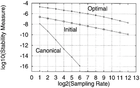
Figure 3 depicts the values of the FWL stability

meas-ure ·1 for the three di erent realizations, Xcan, X0 and

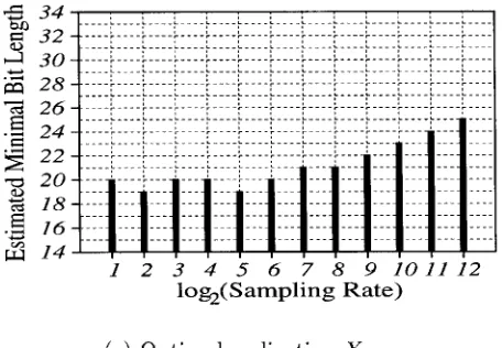
Xopt, under various sampling conditions. Figure 4 shows

the corresponding estimated minimum bit length _B

^

min

s1

[image:9.547.287.524.41.191.2]

that can guarantee the closed-loop stability for these controller realizations. The results clearly show that

(10)

the optimal controller realization has a much larger closed-loop stability margin than the non-optimal initial realization and requires a much smaller word length in ® xed-point implementation. Speci® cally, for this ex-ample, the optimization achieved an improvement by

two orders of magnitude on the stability measure and an average 8-bit reduction in the required minimum bit length over the range of sampling rates. It can also be seen that, for the controllable canonical realization, at

the sampling rate of 26, the stability measure had

already dropped to 10¡16_{, which indicated that the}

closed-loop system with this controller realization was very close to unstable.

6. Conclusions

This paper has presented an optimization procedure for obtaining the optimal realization of ® nite-precision digital controller structures. The procedure possesses the maximum closed-loop stability robustness subject to FWL implemented controller coe cients and requires the minimum bit length in ® xed-point implementation. The approach can be regarded as an extension of an earlier procedure, derived for optimal ® nite-precision PID controller structures, to the general form of sampled-data controller structures. The study has shown that the optimal FWL controller realization problem can be formulated as a constrained nonlinear optimization problem. An e cient global optimization strategy based on the ASA algorithm has been devel-oped to solve this non-smooth and non-convex optimi-zation problem. The theoretical results have been veri® ed using a numerical control system.

Acknowledgments

The third author, J. Wu, would like to thank the National Natural Science Foundation of China under Grant 69504010 and Cao Guangbiao Foundation of Zhejiang University for their ® nancial support.

References

AARTS,E.H.L., andKORST,J.H.M.,1989,Simulated Annealing and Boltzmann Machines(Chichester: Wiley).

BEVERIDGE,G.S.C., and SCHECHTER,R.S.,1970, Optimization: Theory and Practice(McGraw-Hill).

CHEN, T., and FRANCIS, B. A., 1991, Input± output stability of sampled-data systems. IEEE Transactions on Automatic Control, 36,50± 58.

CHEN,S.,LUK,B.L., and LIU,Y.,1998, Application of adaptive simulated annealing to blind channel identi® cation with HOC ® t-ting.Electronics L etters,34, 234± 235.

CHEN,S.,WU,J.,ISTEPANIAN,R.H., andCHU,J.,2000, Optimizing stability bounds of ® nite-precision PID controller structures.IEEE Transactions on Automatic Control, to appear.

DIXON,L.C.W.,1972,Nonlinear Optimisation(London: The English Universities Press Ltd).

FIALHO,I.J., andGEORGIOU,T.T.,1994, On stability and perform-ance of sampled-data systems subject to wordlength constraint. IEEE Transactions on Automatic Control,39,2476± 2481.

GEMAN,S., andGEMAN,D.,1984, Stochastic relaxation, Gibbs distri-bution and the Bayesian restoration in images.IEEE Transactions on Pattern Analysis and Machine Intelligent,6,721± 741.

[image:10.547.33.261.415.573.2]

Optimal® nite-precision controller realization 437

(11)

GEVERS, M., and LI, G., 1993, Parameterizations in Control, Estimation and Filtering Problems: Accuracy Aspects (London: Springer Verlag).

INGBER, L., 1996 , Adaptive simulated annealing (ASA): lessons learned.Journal of Control and Cybernetics,25,33± 54.

INGBER,L., andROSEN,B.E.,1992, Genetic algorithms and very fast simulated reannealing: a comparison. Mathematical and Computer Modelling,16,87± 100.

ISTEPANIAN,R. H.,1997, Implementation issues for discrete PID algorithms using shift and delta operators parameterizations. In Proceedings of the 4th IFAC W orkshop Algorithms and Architectures for Real-Time Control, Vilamoura, Portugal, pp. 117± 122.

ISTEPANIAN,R.H.,PRATT,I.,GOODALL,R., andJONES,S.,1996, E ect of ® xed point parameterization on the performance of active suspension control systems. InProceedings of the 13th IFAC W orld Congress, San Francisco, USA, pp. 291± 295.

ISTEPANIAN,R.H.,LI,G.,WU,J., andCHU,J.,1998a, Analysis of sensitivity measures of ® nite-precision digital controller structures with closed-loop stability bounds. IEE Proceedings for Control Theory and Applications,145,472± 478.

ISTEPANIAN, R. H., WU, J., WHIDBORNE, J. F., YAN, J., and

SALCUDEAN,S.E.,1998b, Finite-word-length stability issues of tele-operation motion-scaling control system. InProceedings of UKACC Control ’98, Swansea, UK, pp. 1676± 1681.

KOWALIK,J., andOSBORNE,M.R.,1968, Methods for Unconstrained Optimization Problems(New York: Elsevier).

LI,G.,1998, On the structure for digital controllers with ® nite word length consideration.IEEE Transactions on Automatic Control,43, 689± 693.

MADIEVSKI,A.G.,ANDERSON,B.D.O., and GEVERS,M.,1995, Optimum realizations of sampled-data controllers for FWL sensitiv-ity minimization.Automatica,31,367± 379.

MORONEY, P., WILLSKY, A. S., and HOUPT, P. K., 1980, The digital implementation of control compensators: the coe cient wordlength issue. IEEE Transactions on Automatic Control, 25, 621± 630.

ROBERTS,R.A., andMULLIS,C.T.,1987,Digital Signal Processing (Addison-Wesley).

ROSEN,B.E.,1997, Rotationally parameterized very fast simulated

reannealing. Submitted to IEEE Transactions on Neural

http://www.informaworld.com/smpp/title~content=t713697751

http://dx.doi.org/10.1080/002077200291019

http://www.informaworld.com/terms-and-conditions-of-access.pdf