Abstract— Monthly counts of industrial machine part errors are modeled using two-state hidden Markov models (HMMs) in order to describe the effect of machine part error correction on the likelihood of the machine parts to be in a “defective” or “non-defective” state. A Bayesian framework is used for parameter estimation. The study finds that the machine part error correction does not improve the machine part status of individual part, but there is a very strong month-to-month dependence of machine part states. A comparison shows that the proposed HMM has a better performance than the traditional Poisson generalized estimating equations (GEE) that directly model the counts.
Index Terms— Hidden Markov Models (HMMs), Machine parts errors, Defective and non-defective state, Bayesian framework
I. INTRODUCTION
ndustrial machine parts data have provided information useful for addressing questions regarding effectiveness of machine part error correction. Using machine part error records, it is possible to collect the number of machine part errors for each part over an entire time period. This data type has been useful in the study of machine part errors. A model for these count data can then be constructed and used to estimate the effect of the machine error correction.
In the study of industrial machine parts, it is reasonable to hypothesize an unobserved machine part state that governs individual errors with the normal error rate corresponding to a “non-defective” state and an excess errors corresponding to “defective” state. The probability of being in the “defective” or “non-defective” state for a particular part in a given month will differ depending on its past state in which that part was in and other possible covariates including specifically error correction. The terms “defective” and “non-defective” are used throughout this paper as labels for the two different states, but it is important to point out that the two states reflect periods of high and low machine errors which are the surrogates for the concepts of “defective” and “non-defective” respectively. As such there may be periods
Manuscript received December 22, 2013; revised January 29, 2014. This work was supported in part by the Department of Manufacturing Systems and Processes, the Faculty of Mechanical Engineering, Technical University of Liberec, Czech Republic.
Pornpit Sirima is with the Department of Manufacturing Systems and Processes, the Faculty of Mechanical Engineering, Technical University of Liberec, Czech Republic (e-mail: [email protected]).
Premysl Pokorny is with the Department of Manufacturing Systems and Processes, the Faculty of Mechanical Engineering, Technical University of Liberec, Czech Republic (corresponding author, phone:+420-48-535-3366; e-mail: [email protected]).
of frequent machine errors corresponding to a “defective” state being predicted by the model that in the reality of the machine part do not represent a “defective” period in the machine part and vice versa for low use and the “non-defective” state.
In this paper we propose the model for “defective” and “non-defective” unobserved machine states as a hidden Markov chain and since the observations are monthly counts of machine part errors, a two-state Poisson hidden Markov model (HMM) [1, 2]is used. The major research question is whether machine part error correction reduces the probability of subsequently entering the “defective” state as measured by the machine part errors.
We consider fitting the two-state hidden Markov model to the number of machine part errors per month. Estimation of parameters for the HMM can proceed within a frequentist or Bayesian framework. Within the maximum likelihood framework, the EM algorithm, also known as the Baum-Welch algorithm in the HMM literature, can be implemented by treating the hidden states as missing values, implementing the forward backward recursion in the E-step and finding the value of the parameters that maximize the likelihood in the M-step [3-4]. Within the Bayesian framework, the MCMC technique and Metropolis-Hastings algorithms can be used to sample from the posterior distribution of the parameters [5]. Reference [6] pointed out that MCMC methods for HMMs can also be improved by incorporating the forward-backward, likelihood and Viterbi recursive algorithms into the MCMC algorithm, improving convergence as well as computational efficiency. While these algorithms can be incorporated to improve the computational efficiency of the MCMC, it is important to note that the direct Gibbs sampling approach for the HMMs is computationally straightforward and intuitive. Moreover, direct Gibbs sampling can be implemented in the existing OpenBUGS software which, in this paper, is used for fitting the data within a Bayesian framework.
The methodology and application are given in section 2, including HMMs, Bayesian models, Gibbs sampling, accessing MCMC convergence, and an application. The results are presented in section 3. Section 4 and 5 give some discussion and conclusion, respectively.
II. METHODOLOGY AND APPLICATION A. Hidden Markov Models
Let ( ,...,1 )T T
y y
=
y be the vector of observed variables, indexed by time. HMMs [7-8] assume that the distribution of
Hidden Markov Models for Analysis of
Defective Industrial Machine Parts
Pornpit Sirima and Premysl Pokorny
each observed data point y depends on an unobserved t (hidden) variable, denoted s, that takes on values from 1 to
k . The hidden variable ( ,...,1 )T T
s s
=
s characterizes the
“state” which the generating process is at any time t. HMMs further postulate a Markov Chain for the evolution of the unobserved state variable and, hence, the process for
t
s is assumed to depend on the past realizations of y and s only through st−1:
1
( t | t ) ij
p s = j s− = =i λ , (1) where λijis the generic element of the transition matrix
(λij)
=
Λ , with vector of stationary probability πsatisfying .
T = T
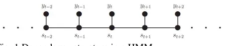
[image:2.595.61.287.296.343.2]π Λ π Figure 1 illustrates the dependency structure in a HMM. Showing that each observation yt is the conditionally independent of all other unobserved and observed data, given st.
Fig. 1 Dependency structure in a HMM
B. Bayesian Models
Suppose y is a vector of observations, y=( ,...,y1 ym), and θ is a vector of parameters,
1
( ,...,θ θk)
=
θ that are not
observable.
For Bayesian models [9], Let f ( | )y θ represent the probability density function of y given θ, and π( )θ is a prior for θ. Then, the posterior probability density function of θ is given by
f ( | )π( ) π( | )
f ( | )π( )d
=
∫
y θ θ
θ y
y θ θ θ
. (2)
The goal of Bayesian inference is to get the posterior. In particular, some numerical summaries may be obtained from the posteriors. For example, to keep things simple, a Bayesian point estimator for a univariate θ is often obtained as the posterior mean:
E( | ) π( | )d
f ( | )π( )d . f ( | )π( )d
θ θ θ θ
θ θ θ θ
θ θ θ
= =
∫
∫
∫
y y y y (3)The posterior variance,var( | )θ y , is often used as Bayesian measure of uncertainty. Markov Chain Monte Carlo (MCMC) methods are proposed to handle the computation.
C. Gibbs Sampling
The Gibbs sampling [10] decomposes the joint posterior distribution into full conditional distributions for each parameter in the model and then sample from them. The sampler can be efficient when the parameters are not highly dependent on each other and the full conditional distributions are easy to sample from. It does not require an instrumental proposal distribution as Metropolis methods do. However, while deriving the conditional distributions can be relatively easy, it is not always possible to find an efficient way to sample from these conditional distributions.
Suppose ( ,...,1 )T k
θ θ
=
θ is the parameter vector, p( | )y θ is the likelihood, and π( )θ is the prior distribution. The full posterior conditional distribution of π(θ θi| j,i≠ j, )y is proportional to the joint posterior density; that is,
π(θ θi | j,i≠ j, )y ∝p( | )y θ π( )θ . For instance, the one-dimensional conditional distribution of θ1 given *
,
j j
θ =θ
2≤ ≤j k, is computed as
* 1
* * * *
1 2 1 2
π( | , 2 , )
p( | ( ( , ,..., ) π( ( , ,..., ) ) .
j j
T T
k k
j k y
θ θ θ
θ θ θ θ θ θ
= ≤ ≤
= = =
y
θ θ
(4)
The Gibbs sampler works as follows:
1. Set
t
=
0
, and choose an arbitrary initial value of θ0 =(θ01,...,θk0).2. Generate each component of θ as follows:
draw ( 1) 1
t
θ + from ( ) ( )
1 2
π( | t ,..., t , )
k
θ θ θ y
draw ( 1) 2
t
θ + from ( 1) ( ) ( )
2 1 3
π( | t , t..., t , )
k
θ θ + θ θ
y
…
draw θk(t+1) from π( | 1(t 1), 3(t 1)..., (t 1), )
k k
θ θ + θ + θ +
y .
3. Set t= +t 1. If
t
<
T
, the number of desired samples, return to step 2. Otherwise, stop.In the MCMC, there are other related processes, called convergence, which are described in the following topics.
D. Assessing MCMC convergence
Simulation-based Bayesian inference requires using simulated draws to summarize the posterior distribution or calculate any relevant quantities of interest. We have to decide whether the Markov chain has reached its stationary, or the desired posterior distribution and to determine the number of iterations to keep after the Markov chain has reached stationarity. Convergence diagnostics help to resolve these issues. Reference [11] discuss about convergence diagnostics. The common ones are visual analysis via trace plots and kernel density plots.
E. An Application
from January 2012 to November 2012. The number of machine parts errors were recorded.
A Hidden Markov model for the number of machine part errors Zit is
( )
|it it it
Z θ Pois θ
0 1
log(θit)=λ +λCit (5)
1
( 1) 0 1 ( 1) 2
| Bin(logit ( ),1)
it i t i t it
C C − − β +βC − +β X
0 Bin(1, 1)
it
C π
where θit, which can be viewed as the mean of the Poisson, is determined by the unobserved machine part state Cit. This unobserved machine parts state follows a Markov chain, with transition probability modeled by a logistic regression with the previous health state Ci t(−1). The parameter π1 represents the initial probability of being in the “defective” machine state at the first month ti1, i.e.
1
Pr( 1) i
it
C = . The dummy variables Xit =1 indicates the status of month t for part ias being after error correction (with before correction as the reference group, Xit =0 ). Thus, the estimate for the coefficient of Xit is of primary interest to see if the probability of being in the “defective” state has significantly decreased after correction.
The hidden Markov model (5) is illustrated in Figure 1. The total number of machine parts error Zit in a particular month t, is governed by the two state latent variable Cit. More specifically, Zit comes from a two state Poisson distribution where the two different means of the Poisson distribution correspond to the two different values of the latent variable Cit which in turn depends on the previous state Ci t(−1). To make the unobserved states identifiable, we assume that the lower mean corresponds to Cit =0 and the higher mean corresponds to Cit =1, which is operationalized by constraining λ1to be larger than zero. Thus
0
it
C = corresponds to the “non-defective” state and 1
it
C = corresponds to the “defective” state.
F. Parameter Estimation
The MCMC Gibbs sampling for parameter estimation was done in a Bayesian framework using MCMC techniques via OpenBUGS software. The joint posterior is broken into the full conditional posterior distribution with respect to each parameter and the Gibbs sampler [18] is used. Once the chain converges, the empirical joint posterior distribution for all the parameters can be used to obtain the posterior mean and the 2.5% and 97.5% quantiles can be used as the credible interval for all the parameters. The priors were chosen to be as noninformative as possible. In the total visits model, N(0,10 )5 priors were used for λ0,β0,β1,β2, and N(0,10 )5 with positive value restriction was used for
1 λ .
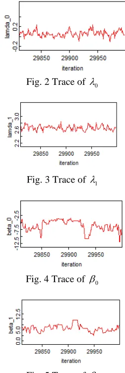
The visual analysis, history plots and kernel density plots are used for the MCMC convergence diagnostics. We performed 25,000 MCMC iterations with 5,000 burn-in iterations.
To evaluate the model performance, the proposed model is compared with the traditional Poisson generalized estimating equations (GEE) that directly model the counts, using mean square errors (MSE).
The GEE is expressed as:
( )
|it it it
Z θ Pois θ
0 1
log(θit)=β +β Xit , (5) where β0 and β1are regression coefficients, the dummy variables Xit =1 indicates the status of month t for part ias being after error correction. We use SPSS software for the GEE parameter estimation.
III. RESULTS
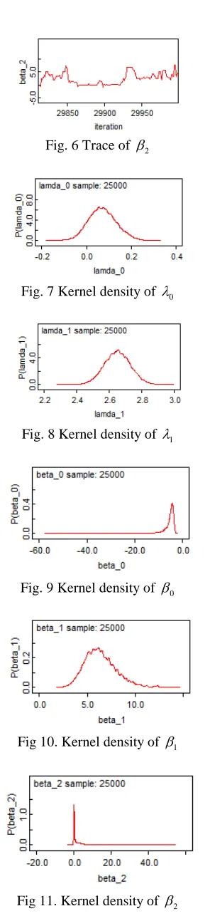
[image:3.595.368.494.397.773.2]The mean number of machine part error was 2.35 per one part per one month. As the observed data represent the count of machine parts errors, direct modeling of the data via GEE is considered. The visual analysis is used for MCMC convergence diagnostics. The trace plots are shown in Fig. 2-6 and the kernel density plots are shown in Fig. 7-11. The chains moving around the parameter spaces and the kernel densities looking like their distributions indicate that each parameter is converged to a stationary density.
Fig. 2 Trace of λ0
Fig. 3 Trace of λ1
Fig. 4 Trace of β0
Fig. 6 Trace of β2
Fig. 7 Kernel density of λ0
Fig. 8 Kernel density of λ1
Fig. 9 Kernel density of β0
[image:4.595.104.252.38.681.2]Fig 10. Kernel density of β1
Fig 11. Kernel density of β2
The posterior summary of the estimated parameters is shown in Table 1.
TABLE I
PARAMETER ESTIMATES FROM THE HMM Parameter Mean SD 95% Credible Interval
0
λ 0.071 0.063 -0.045 0.198
1
λ 2.649 0.080 2.492 2.808
0
β -5.469 2.491 -12.08 -3.336
1
β 6.393 1.66 3.655 10.14
2
β 1.284 2.593 -0.3057 7.868
Table 1 shows the results of the HMM fit to the machine part error counts per month. The estimate of β2(1.284) implies that the odds of transitioning to or remaining in the “defective” state in any given month after correction is exp(1.284) = 3.611 of what it was before correction. This provides evidence in favor of the machine part error correction not improving the machine part status of individual part.
In addition to this main finding, the results from the model also characterize a very strong month-to-month dependence of machine part states (β1= 6.393) where the odds of remaining in the “defective” state in the current month if an machine part was in the “defective” state the last month is estimated to be exp(6.393) = 597.647 times the odds of newly transitioning to the “defective” state if an individual part was “non-defective” in the previous month.
For the model comparison, the mean square errors (MSE) of the proposed HMM (3.193) is smaller than the GEE (4.948), indicating that it has a better performance.
IV. DISCUSSION
We propose a HMM for machine part errors. The model assumes there are unobserved machine part states that govern the machinery care utilization of a particular machine part, and the machine part state is governed only by the frequency of errors.
The main goal of the HMM is to model changing machine part states over time not necessarily modeling the changing number of errors. In the HMM, the observed machine errors are really only a surrogate for “machine parts status”. Measurement error is allowed between the observed machine errors and the underlying machine state. For the GEE, the goal is to model the changing numbers of machine part themselves. As being seen from the model comparison using mean square errors (MSE), the GEE does not fit as well. Reference [12] give a review and description of several different Markov and latent (hidden) Markov models. The proposed HMMs can be applied to other similar problems and can be extended to multivariate Poisson data.
V. CONCLUSION
The objective of this study is to propose a two-state hidden Markov model in order to describe the effect of machine part error correction on the likelihood of the machine parts to be in a “defective” or “non-defective” state. A Bayesian framework is used for parameter estimation. The study finds that the machine part error correction does not improve the machine part status of individual part, and there is a very strong month-to-month dependence of machine part states. Using root mean square errors, the proposed HMM is compared to the GEE that directly model the counts. The results show that the proposed model has a better performance.
REFERENCES
[1] W. M. Melanie, and L. Ran, “Multiple indicator hidden Markov model with an application to medical utilization data,” Stat Med, vol. 28 no.2, pp. 293–310, 2009.
[2] I. L. MacDonald, and W. Zucchini, Hidden Markov and other
Models for Discrete-valued Time Series. New York: Chapman and
Hall, 1997.
[3] L. E. Baum, T. Petrie, G. Soules, and N. Weiss, “A maximization technique occurring in the statistical analysis of probabilistic functions of Markov chains,” The Annuals of Mathematical
Statistics, vol. 41, pp. 164–171, 1970.
[4] J. A. Bilmes, “A Gentle Tutorial of the EM Algorithm and its Application to Parameter Estimation for Gaussian Mixture and Hidden Markov Models,” Technical Report, University of Berkeley,
ICSITR, pp. 97-121, 1998.
[5] J. H. Albert, S. Chib, “Bayes Inference via Gibbs Sampling of Autoregressive Time Series Subject to Markov Mean and Variance Shifts,” Journal of Business and Economic Statistics, vol. 11, pp. 1– 15, 1993.
[6] S. L. Scott, “Bayesian Methods for Hidden Markov Models: Recursive Computing in the 21st Century,” Journal of the American
Statistical Association, vol. 97, pp. 337–351, 2002.
[7] A. M. Poritz, “Hidden Markov models: a guided tour,” Proceedings
of the IEEE International Conference on Acoustics, Speech and Signal Processing , vol. 1, pp. 7-13, 1988.
[8] L. R. Rabiner, “A tutorial on hidden Markov models and selected applications in speech recognition,” Proceedings of the IEEE, vol. 77, pp. 257-285, 1989.
[9] P. Congdon, Bayesian Statistical Modelling. 2nd ed. New York: John Wiley and Sons, 2006.
[10] S. Geman, D. Geman, “Stochastic Relaxation Gibbs Distributions, and the Bayesian Restoration of Images,” IEEE Transactions of
Pattern Analysis and Machine Intelligence, vol. 6, pp. 721-74, 1984.
[11] S. P. Brooks, and G. O. Roberts, “Assessing Convergence of Markov Chain Monte Carlo Algorithms,” Statistics and Computing, vol. 8, pp. 319-335, 1998.
[12] R. Langeheine, F. van de Pol, Latent Markov Chains, Applied Latent