Multilayer Perceptron Learning Utilizing
Singular Regions and Search Pruning
Seiya Satoh and Ryohei Nakano
Abstract—In a search space of a multilayer perceptron having J hidden units, MLP(J), there exist flat areas called singular regions. Since singular regions cause serious stagnation of learning, a learning method to avoid them was once proposed, but was not guaranteed to find excellent solutions. Recently, SSF1.2 was proposed which utilizes singular regions to stably and successively find excellent solutions commensurate with MLP(J). However, SSF1.2 has a problem that it takes longer as J gets larger. This paper proposes a learning method SSF1.3 that enhances SSF1.2 by attaching search pruning so as to discard a search whose route is similar to one of previous searches. Our experiments showed SSF1.3 ran several times faster than SSF1.2 without degrading solution quality.
Index Terms—multilayer perceptron, learning method, sin-gular region, reducibility mapping, search pruning
I. INTRODUCTION
In a parameter space of MLP(J), a multilayer perceptron with J hidden units, there exist flat areas called singular regions created by reducibility mapping [1], and such a region causes stagnation of learning [2]. Hecht-Nielsen once pointed out MLP parameter space is full of flat areas and troughs [3], and recent experiments [4] revealed most points have huge condition numbers (>106).
Natural gradient [5] was once proposed to avoid singular regions, but even the method may get stuck in singular regions and is not guaranteed to find an excellent solution.
It is known that many useful statistical models, such as MLP, GM, and HMM, are singular models having singular regions. Intensive theoretical research has been done to clar-ify mathematical features of singular models and especially Watanabe has produced his own singular learning theory [6]; however, experimental research has been rather insufficient so far to fully support the theories.
Recently a rather unusual learning method called SSF (Singularity Stairs Following) [4], [7] was proposed for MLP learning, which does not avoid but makes good use of singu-lar regions of MLP search space. The latest version SSF1.2 [7] successively and stably finds excellent solutions, starting with MLP(J=1) and then gradually increases J. When increasing J, SSF1.2 utilizes the optimum of MLP(J−1) to form two kinds of singular regions in MLP(J) parameter space. Thus, SSF1.2 can monotonically improve the solution quality along with the increase of J. The processing time of SSF1.2, however, gets very long as J gets large due to the increase of search routes. Moreover, it was observed that many SSF runs converged into very limited number of solutions, indicating the great potential for search pruning.
This work was supported in part by Grants-in-Aid for Scientific Research (C) 25330294 and Chubu University Grant 24IS27A.
S. Satoh and R. Nakano are with the Department of Computer Science, Graduate School of Engineering, Chubu University, 1200 Matsumoto-cho, Kasugai 487-8501, Japan. email: [email protected] and [email protected]
This paper proposes a learning method called SSF1.3 which enhances SSF1.2 by attaching search pruning so as to prune any search going through a route similar to one of previous searches. Our experiments using artificial and real data sets showed SSF1.3 ran several times faster than SSF1.2 without degrading solution quality.
II. SINGULARREGIONS OFMULTILAYERPERCEPTRON This section explains how the optimum of MLP(J−1) can be used to form singular regions in MLP(J) parameter space [2], [7]. Hereafter the boldface indicates a vector.
Consider MLP(J) having J hidden units and one output unit. MLP(J) having parameters θJ outputs fJ(x;θJ) for input vectorx= (xk). Letx beK-dimensional.
fJ(x;θJ) =w0+
J ∑
j=1
wjzj, zj≡g(wTjx) (1)
Hereg(h)is an activation function and aT is the transpose ofa;θJ={w0, wj,wj, j= 1,· · ·, J}, wherewj = (wjk). Given training data {(xµ, yµ), µ = 1,· · ·, N}, we con-sider findingθJ that minimizes the following error function.
EJ=
1 2
N ∑
µ=1
(fJµ−yµ)2, fJµ≡fJ(xµ;θJ) (2)
Moreover we consider MLP(J−1) havingJ−1 hidden units and one output unit. MLP(J−1) with parameters θJ−1 =
{u0, uj,uj, j= 2,· · ·, J} outputs the following:
fJ−1(x;θJ−1) =u0+
J ∑
j=2
ujvj, vj ≡g(uTjx). (3)
The error function of MLP(J−1) is defined as follows.
EJ−1(θ) = 1 2
N ∑
µ=1
(fJµ−1−yµ)2 (4)
Here fJµ−1 ≡ fJ−1(xµ;θJ−1). Then, let θbJ−1 =
{bu0,ubj,ubj, j= 2,· · ·, J} be the optimum of MLP(J−1). Now we introduce the following reducibility mappingsα,
β,γ, and letΘbαJ,Θb β J, andΘb
γ
J denote the regions obtained by applying these three mappings to the optimum bθJ−1 of
MLP(J−1). Here letm= 2,· · ·, J in the last mapping. b
θJ−1
α
−→ΘbαJ, θbJ−1
β
−→ΘbβJ, bθJ−1
γ
−→ΘbγJ (5)
b
ΘαJ ≡ {θJ|w0=bu0, w1= 0,
wj =buj,wj=ubj, j= 2,· · ·, J} (6) b
ΘβJ ≡ {θJ|w0+w1g(w10) =bu0, w1= [w10,0,· · ·,0]T,
wj =buj,wj=ubj, j= 2,· · ·, J} (7) b
ΘγJ ≡ {θJ|w0=bu0, w1+wm=ubm, w1=wm=ubm,
By checking the necessary conditions for the critical point of MLP(J), we have the following result [7], which means there are two kinds of singular regions ΘbαβJ and Θb
γ J in MLP(J) parameter space.
(1) RegionΘbαJ is (K+ 1)-dimensional since free vectorw1
is (K+ 1)-dimensional. In this region since w1 is free, the
output of the first hidden unit z1µ is free, which means the necessary conditions do not always hold. Thus,ΘbαJ is not a singular region in general.
(2) RegionΘbβJis two-dimensional since all we have to do is to satisfyw0+w1g(w10) =ub0.In this regionz1µ(=g(w10))
is independent onµ; however, some necessary condition does not hold in general unlessw1= 0. Thus, the following area
included in bothΘbαJ andΘbβJ forms a singular region where onlyw10 is free. The region is calledΘb
αβ
J and reducibility mapping frombθJ−1 toΘb
αβ
J is calledαβ.
w0=bu0, w1= 0, w1= [w10,0,· · ·,0]T,
wj =ubj, wj=ubj, j= 2,· · ·, J (9)
(3) RegionΘbγJ is a line since we have only to satisfyw1+ wm =bum. In this region all the necessary conditions hold since zµ1 =vµ
m. Namely,Θb γ
J is a singular region. Here we have a line since we only have the following restriction.
w1+wm=bum (10)
III. SINGULARITYSTAIRSFOLLOWING
This section explains the framework of SSF (singularity stairs following) [4], [7]. SSF is a search method which makes good use of singular regions.
Here, we consider the following four technical points of SSF. SSF1.2 [7] and the proposed SSF1.3 share the first three points, but they are different in the last point.
The first point is on search areas; that is, SSF1.2 and 1.3 search whole two kinds of singular regions ΘbαβJ and ΘbγJ. By searching the whole singular regions, SSF1.2 and 1.3 will find better solutions than SSF1.0 [4].
The second point is how to start search from singular regions. Since a singular region is flat, any method based on gradient cannot move. Thus, SSF1.0 employs weak weight decay, distorting the original search space, while SSF1.2 and 1.3 employ the Hessian H(=∂2E/∂w∂wT). Figure 1 illustrates an initial point on the singular region. Since most points in singular regions are saddles [2], we surely find a descending path which corresponds to a negative eigen value ofH. That is, each negative eigen value ofHis picked up, and its eigen vector v and its negative −v are selected as two search directions. The appropriate step length is decided using line search [8]. After the first move, the search is continued using a quasi-Newton called BPQ [9].
The third point is on the number of initial search points; namely, SSF1.2 and 1.3 start search from singular regions in a very selective way, while SSF1.0 tries many initial points in a rather exhaustive way. As for regionΘbγJ, SSF1.2 and 1.3 start from three initial points: a middle interpolation point, a boundary point, and an extrapolation point. These correspond toq=0.5, 1.0, and 1.5 respectively in the following. Note that the restriction eq. (10) is satisfied.
w1=q bum, wm= (1−q)ubm (11)
E
[image:2.595.367.482.63.143.2]a starting point
Fig. 1. Conceptual diagram of a singular region.
On the other hand, SSF1.0 exhaustively tries many initial points in the form of interpolation or extrapolation of eq.(10). As for regionΘbαβJ , SSF1.2 and 1.3 use only one initial point in the region, while SSF1.0 does not search this region.
The final point is on search pruning, which is newly introduced in SSF1.3; neither SSF1.0 nor SSF1.2 has such feature. Our previous experiences on SSF indicated that although we started many searches from singular regions, we obtained only limited kinds of solutions. This means many searches join together through their search processes. Thus, we consider the search pruning described below will surely accelerate the whole search.
Now our search pruning is described in detail. Let θ(t)
andφ(i)be a current search node and a previous search node respectively. Here a search node means a search point to be checked or recorded at certain intervals, say at every 100 moves. We introduce the following normalization of weights in order to make the pruning effective. The normalization will prevent large weight values from overly affecting the similarity judging. Letdbe a normalization vector.
dm ←
{
1/|θm(t−1)| (1<|θm(t−1)|)
1 (|θ(mt−1)| ≤1)
(12)
v(t) ← diag(d)θ(t) (13)
v(t−1) ← diag(d)θ(t−1) (14)
r(i) ← diag(d)φ(i), i= 1,· · ·, I (15)
Herem= 1,· · ·, M, andM is the number of weights.I is the number of previous search nodes stored in memory, and diag(d) denotes a diagonal matrix whose diagonal elements ared and the other elements are zero.
r(i)
v(t)
r(i−1)
l v(t−1)
v(t−2)
r(i−2)
r(i−3)
[image:2.595.333.548.453.529.2]r(i−4)
Fig. 2. Conceptual diagram of search pruning.
Figure 2 illustrates a conceptual diagram of search prun-ing. We consider previous line segment vectors fromr(i−1)
[image:2.595.371.490.602.683.2]close enough to any previous line segment, then the current search is pruned at once. We define two difference vectors ∆r(i) ≡ r(i)−r(i−1), and ∆v(t) ≡ v(t)−v(t−1). Then
consider a segment vector perpendicular to both lines which include the above difference vectors. The segment vector is described as below.
`= (r(i−1)+a14r(i))−(v(t−1)+a24v(t)) (16)
Unknown variables a ≡ (a1, a2)T can be determined by
solving the following minimization problem.
min
a `
T
` (17)
The solutionacan be written as below. Hereb1≡ k4r(i)k2, b2 ≡ 4r(i)T4v(t), b3 ≡ k4v(t)k2, b4 ≡ (r(i−1)− v(t−1))T4r(i),b5≡(r(i−1)−v(t−1))T4v(t).
a = − 1
b1b3−b22
[
b3b4−b2b5 b2b4−b1b5
]
(18)
Both endpoints of the line segment ` are on two difference vectors ∆r(i) and ∆v(t) if and only if the following equations hold.
0≤a1≤1, 0≤a2≤1 (19)
If both of the above hold and each element`mof `satisfies
`m < , then we consider the current search joins some previous search, and prune it. Otherwise, we consider the current search is different from any previous searches. In our experiments we set = 0.3.
The procedure of SSF1.3 is described below, which is much the same as that of SSF1.2. The only difference is presence or absence of search pruning. SSF1.3 searches MLP parameter spaces by ascending singularity stairs one by one, beginning with J=1 and gradually increasingJ until Jmax. The optimal MLP(J=1) can be found just applying reducibil-ity mapping αβ to the optimal MLP(J=0); MLP(J=0) is a constant model. Step 1 embodies such search. Step 2-1 and step 2-2 search MLP(J+1) parameter space starting from singular regions ΘbαβJ+1, and Θb
γ
J+1 respectively. Here w (J) 0 , w(jJ), andw(jJ) denote weights of MLP(J).
SSF1.3 (Singularity Stairs Following, ver. 1.3):
(step 1) Initialize weights of MLP(J=1) using reducibility mapping αβ:
w(1)0 ←wb0(0)=y, w1(1)←0, w(1)1 ←[0,0,· · ·,0]T. Pick up each negative eigen value of the Hessian H and select its eigen vector v and −v as two search directions. Find the appropriate step length using line search. Then perform MLP(J=1) learning with search pruning and keep the best as wb0(1),wb1(1), andwb(1)1 .J←2.
(step 2) While J < Jmax, repeat the following to get the optimal MLP(J+1) from the optimal MLP(J).
(step 2-1) Initialize weights of MLP(J+1) applying re-ducibility mappingαβ to the optimal MLP(J):
wj(J+1)←wbj(J), j= 0,1,· · ·, J,
w(jJ+1)←wb(jJ), j= 1,· · ·, J
wJ(J+1+1)= 0, w(JJ+1+1)←[0,0,· · ·,0]T.
Find the reasonable search directions and their appropriate step lengths by using the procedure shown in step 1. Then perform MLP(J+1) learning with search pruning and keep
the best as the best MLP(J+1) ofαβ.
(step 2-2)If there are more than one hidden units in MLP(J), repeat the following for each hidden unitm(= 1,· · ·, J)to split.
Initialize weights of MLP(J+1) using reducibility mapping
γ:
wj(J+1)←wbj(J), j∈ {0,1,· · ·, J} \ {m},
w(jJ+1)←wb(jJ), j= 1,· · ·, J
w(JJ+1+1)←wb(mJ).
Initialize w(mJ+1) and w(JJ+1+1) three times as shown below withq= 0.5, 1.0, and 1.5.
wm(J+1)=q wb
(J)
m , w
(J+1)
J+1 = (1−q)wb (J)
m
For each of the above three, find the reasonable search directions and their appropriate step lengths by using the procedure shown in step 1. Then perform MLP(J+1) learning with search pruning and keep the best as the best MLP(J+1) ofγ for m.
(step 2-3) Among the best MLP(J+1) of αβ and the best MLP(J+1)s of γ for different m, select the true best and let the weights bewb(0J+1),wb(jJ+1),wb(jJ+1),j =1,· · ·, J+1. ThenJ ←J+1.
Now we claim the following, which will be evaluated in our experiments.
(1) Compared with existing methods such as BP, quasi-Newtons, SSF1.3 will find excellent solutions with much higher probabilities.
(2) Excellent solutions will be obtained one after another for
J =1,· · ·, Jmax. SSF1.3 guarantees the monotonic improve-ment of training solution quality, which is not guaranteed for most existing methods.
(3) SSF1.3 will be faster than SSF1.0 or SSF1.2 due to the search pruning. SSF1.3 will also be faster than most existing methods if they are performed many times changing initial weights.
IV. EXPERIMENTS
We evaluated the proposed SSF1.3 for sigmoidal and polynomial MLPs using artificial and real data sets. We used a PC with Intel Core i7-2600 (3.4GHz). Forward calculations of sigmoidal and polynomial MLPs are shown in eq. (20) and eq. (21) respectively.
f = w0+
J ∑
j=1
wjzj, zj=σ(wTjx) (20)
f = w0+
J ∑
j=1 wjzj,
zj = K ∏
k=1
(xk)wjk = exp( K ∑
k=1
wjklnxk) (21)
For comparison, we employed batch BP and a quasi-Newton called BPQ [9] as existing methods. The learning rate of batch BP was adaptively determined using line search. BP or BPQ was performed 100 times for each J changing initial weights; i.e., wjk andwj were randomly selected from the range [−1,+1] except w0=y. SSF or BPQ stops when a
test data points independent of training data. For real data 10-fold cross-validation was used, and eachxk andy were normalized asxk/max(xk)and(y−y)/std(y)respectively.
Experiment of Sigmoidal MLP using Artificial Data 1 An artificial data set for sigmoidal MLP was generated using MLP having the following weights. Values of each input variable x1, x2,· · ·, x10 were randomly selected from
the range[0,+1], while values ofywere generated by adding small Gaussian noiseN(0, 0.052)to MLP outputs. Note that five variablesx6,· · ·, x10 are irrelevant. The size of training
data was N= 1,000, andJmax was set to be 8.
(w0, w1, w2, w3, w4, w5, w6)
= (−6,−6,−5,−3,2,10,9), (22)
(w1,w2,w3,w4,w5,w6)
=
−1 −1 1 −3 3 −6
0 7 −9 9 1 4
6 −5 8 −8 −8 3
−9 5 6 3 −4 5
−9 −1 7 −10 −6 −1
9 7 3 −7 −2 6
0 0 0 0 0 0
..
. ... ... ... ... ...
0 0 0 0 0 0
(23)
Table I shows the numbers of sigmoidal MLP search routes of SSF1.2 and 1.3 for artificial data 1. For SSF1.3, initial and final routes correspond to search routes before and after search pruning respectively. For SSF1.3, the total numbers of initial and final routes were 908 and 392 respectively, meaning 56.8 % of initial routes were pruned on their ways.
TABLE I
NUMBERS OF SIGMOIDALMLPSEARCH ROUTES FOR ARTIFICIAL DATA1
J SSF1.2 SSF1.3 initial routes final routes
1 5 5 5
2 29 29 21
3 65 65 48
4 83 83 44
5 122 122 49
6 161 165 76
7 195 200 80
8 245 239 69
[image:4.595.331.522.85.484.2]total 905 908 392
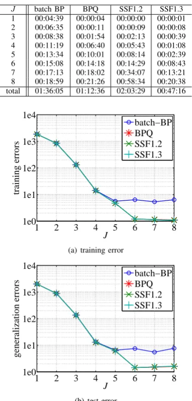
Table II shows CPU time required by each method for sigmoidal MLP using artificial data 1. SSF1.3 was 2.61 times faster than SSF1.2 owing to search pruning. SSF1.3 finished search the fastest among the four.
Figure 3 shows how training and test errors changed along with the increase ofJ. BP stopped decreasing atJ = 5, while SSF and BPQ monotonically decreased training error. As for test error, BP selected J = 7 as the best model, while SSF and BPQ indicatedJ = 6 is the best, which is correct.
Figure 4 compares histograms of BPQ and SSF1.3 solu-tions for MLP(J=6). BPQ found the excellent solution only once out of 100 runs, while SSF1.3 found it eight times out of 97 search routes. Moreover, BPQ solutions are widely scattered, while SSF1.3 solutions are densely located around
TABLE II
CPUTIME FOR SIGMOIDALMLPUSING ARTIFICIAL DATA1 (HR:MIN:SEC)
J batch BP BPQ SSF1.2 SSF1.3 1 00:04:39 00:00:04 00:00:00 00:00:01 2 00:06:35 00:00:11 00:00:09 00:00:08 3 00:08:38 00:01:54 00:02:13 00:00:39 4 00:11:19 00:06:40 00:05:43 00:01:08 5 00:13:34 00:10:01 00:08:14 00:02:39 6 00:15:08 00:14:18 00:14:29 00:08:43 7 00:17:13 00:18:02 00:34:07 00:13:21 8 00:18:59 00:21:26 00:58:34 00:20:38 total 01:36:05 01:12:36 02:03:29 00:47:16
1 2 3 4 5 6 7 8
1e0 1e1 1e2 1e3 1e4
training errors
J
batch−BP BPQ SSF1.2 SSF1.3
(a) training error
1 2 3 4 5 6 7 8
1e0 1e1 1e2 1e3 1e4
generalization errors
J
batch−BP BPQ SSF1.2 SSF1.3
(b) test error
Fig. 3. Training and test errors of sigmoidal MLP for artificial data 1
the excellent solution. The tendencies that SSF1.3 finds excellent solutions with much higher probability and SSF1.3 solutions are more densely located close to an excellent solution were observed in other experiments, which are omitted due to space limitation.
1e0.5 1e1 1e1.5 1e2 1e2.5 0
10 20 30 40 50 60 70 80 90 100
MLP(6)
frequency
E
(a) BPQ
1e0.5 1e1 1e1.5 1e2 1e2.5 0
10 20 30 40 50 60 70
MLP(6)
frequency
E
[image:4.595.85.253.500.604.2](b) SSF1.3
Fig. 4. Histograms of sigmoidal MLP(J=6) solutions for artificial data 1.
[image:4.595.312.543.613.720.2]while values of y were generated by adding small Gaus-sian noise N(0,0.052) to MLP outputs. Here five variables x11,· · ·, x15 are irrelevant. The size of training data was N = 1,000.Jmaxwas set to be 8.
y = 3−50x31x42−28x92x63−23x104 x105 x56−18x47x48
−12x68x109 + 36x10 (24)
Table III shows the numbers of sigmoidal MLP search routes of SSF1.2 and 1.3 for artificial data 2. For SSF1.3, the total numbers of initial and final routes were 1432 and 610 respectively, meaning 57.4 % of initial routes were pruned on their ways.
TABLE III
NUMBERS OF POLYNOMIALMLPSEARCH ROUTES FOR ARTIFICIAL DATA2
J SSF1.2 SSF1.3 initial routes final routes
1 14 14 13
2 47 47 10
3 93 103 41
4 159 146 59
5 210 194 81
6 261 265 97
7 324 274 108
8 386 389 201
total 1494 1432 610
Table IV shows CPU time required by each method for sigmoidal MLP using artificial data 2. SSF1.3 was 2.37 times faster than SSF1.2 owing to search pruning. SSF1.3 finished search the fastest among the four.
TABLE IV
CPUTIME FOR POLYNOMIALMLPUSING ARTIFICIAL DATA2 (HR:MIN:SEC)
J batch BP BPQ SSF1.2 SSF1.3 1 00:03:34 00:02:46 00:00:05 00:00:03 2 00:04:18 00:02:18 00:01:09 00:00:10 3 00:05:20 00:03:01 00:00:59 00:00:40 4 00:06:24 00:03:23 00:03:18 00:01:59 5 00:07:24 00:05:17 00:08:27 00:04:02 6 00:07:28 00:05:38 00:13:13 00:03:55 7 00:08:16 00:06:48 00:21:28 00:08:10 8 00:08:43 00:07:03 00:20:51 00:10:21 total 00:51:27 00:36:15 01:09:32 00:29:22
Figure 5 shows how training and test errors changed when J was increased. BP could not decrease training error efficiently, while SSF and BPQ monotonically decreased at a steady pace. Specifically, SSF outperformed BPQ atJ=6. As for test error, BP stayed at the same level, and BPQ reached the bottom at J = 5 and 6, and rose sharply for J ≥ 7, while SSF1.3 showed a steady move and indicatedJ = 6is the best model, which is correct.
Experiment of Sigmoidal MLP using Real Data
As real data for sigmoidal MLP we used concrete com-pressive strength data from UCI ML repository. The number of input variables is 8, and the data size isN = 1,030. From our preliminary experiment,Jmaxwas set to be 18.
Table V shows the numbers of sigmoidal MLP search routes of SSF1.2 and 1.3 for concrete data. For SSF1.3, the total numbers of initial and final routes were 5523 and 981 respectively, meaning 82.2 % of initial routes were pruned on their ways.
1 2 3 4 5 6 7 8
1e−1 1e0 1e1 1e2 1e3 1e4 1e5
training errors
J batch−BP BPQ SSF1.2 SSF1.3
(a) training error
1 2 3 4 5 6 7 8
1e0 1e5 1e10 1e15 1e20
generalization errors
J batch−BP BPQ SSF1.2 SSF1.3
(b) test error
Fig. 5. Training and test errors of polynomial MLP for artificial data 2
TABLE V
NUMBERS OF SIGMOIDALMLPSEARCH ROUTES USING CONCRETE DATA
J SSF1.2 SSF1.3 initial routes final routes
1 6 6 6
2 30 30 9
3 62 51 14
4 101 87 24
5 107 103 36
6 145 139 44
7 226 176 40
8 209 223 49
9 211 275 75
10 329 422 75
11 300 329 64
12 377 411 84
13 332 484 88
14 340 547 89
15 665 429 68
16 467 692 68
17 612 500 75
18 476 619 73
total 4995 5523 981
Table VI shows CPU time required by each method for sigmoidal MLP using concrete data. SSF1.3 was 4.06 times faster than SSF1.2 owing to search pruning. Again, SSF1.3 finished search the fastest among the four.
TABLE VI
CPUTIME FOR SIGMOIDALMLPUSING CONCRETE DATA(HR:MIN:SEC)
J batch BP BPQ SSF1.2 SSF1.3 1 00:05:40 00:00:05 00:00:00 00:00:01 2 00:07:14 00:07:40 00:02:01 00:00:23 3 00:09:25 00:10:22 00:06:06 00:01:34 4 00:12:33 00:13:38 00:09:00 00:03:53 5 00:14:59 00:16:27 00:16:11 00:06:22 6 00:16:48 00:18:39 00:25:17 00:08:51 7 00:19:04 00:21:28 00:45:15 00:10:10 8 00:21:07 00:23:56 00:46:36 00:15:05 9 00:23:46 00:26:47 00:52:35 00:23:12 10 00:16:18 00:20:17 01:02:19 00:19:01 11 00:18:39 00:23:16 01:03:56 00:18:13 12 00:20:49 00:26:10 01:31:29 00:27:22 13 00:23:08 00:29:18 01:30:04 00:32:26 14 00:25:13 00:32:10 01:42:01 00:37:02 15 00:27:31 00:35:11 03:40:07 00:30:21 16 00:22:53 00:31:52 02:19:24 00:28:05 17 00:24:17 00:34:22 03:17:28 00:31:36 18 00:24:16 00:34:55 02:39:15 00:34:01 total 05:33:37 06:46:31 22:09:05 05:27:35
2 4 6 8 10 12 14 16 18
1e1.2 1e1.4 1e1.6 1e1.8
training errors
J
batch−BP BPQ SSF1.2 SSF1.3
(a) training error
2 4 6 8 10 12 14 16 18
1e1.4 1e1.6 1e1.8
generalization errors
J
batch−BP BPQ SSF1.2 SSF1.3
(b) test error
Fig. 6. Training and test errors of sigmoidal MLP for concrete data
V. CONCLUSION
This paper proposed a new MLP learning method called SSF1.3, which makes good use of the whole singular re-gions and has the search pruning feature. Beginning with MLP(J=1) it gradually increases J one by one to successively and stably find excellent solutions for each J. Compared with existing methods such as BP or a quasi-Newton method, SSF1.3 successively and more stably found excellent solu-tions commensurate with each J. In the future we plan to apply our method to model selection for singular models since successive excellent solutions for each J and learning processes can be used for such model selection.
Acknowledgments.: This work was supported by
Grants-in-Aid for Scientific Research (C) 25330294 and Chubu University Grant 24IS27A.
REFERENCES
[1] H. J. Sussmann, “Uniqueness of the weights for minimal feedforward nets with a given input-output map,”Neural Networks, vol. 5, no. 4, pp. 589–593, 1992.
[2] K. Fukumizu and S. Amari, “Local minima and plateaus in hierarchical structure of multilayer perceptrons,”Neural Networks, vol. 13, no. 3, pp. 317–327, 2000.
[3] H. Hecht-Nielsen,Neurocomputing. Addison-Wesley, 1990. [4] R. Nakano, S. Satoh, and T. Ohwaki, “Learning method utilizing
singular region of multilayer perceptron,” in Proc. 3rd Int. Conf. on Neural Computation Theory and Applications, 2011, pp. 106–111. [5] S. Amari, “Natural gradient works efficiently in learning,” Neural
Computation, vol. 10, no. 2, pp. 251–276, 1998.
[6] W. S.,Algebraic geometry and statistical learning theory. Cambridge University Press, 2009.
[7] S. Satoh and R. Nakano, “Fast and stable learning utilizing singular regions of multilayer perceptron,” Neural Processing Letters, 2013, online DOI:10.1007/s11063-013-9283-z.
[8] D. G. Luenberger, Linear and nonlinear programming. Addison-Wesley, 1984.