Abstract—Nowadays, the amount of available multimedia data is continuously on the rise. The need to find a required image for an ordinary user is a challenging task. Traditional methods as content-based image retrieval (CBIR) compute relevance based on the visual similarity of low-level image features such as color, textures, etc. However, there is a gap between low-level visual features and semantic meanings required by applications. The typical method of bridging the semantic gap is through the automatic image annotation (AIA) that extracts semantic features using machine learning techniques. In this paper, we propose a novel attempt for multi-instance multi-label image annotation (MIML). Firstly, images are segmented by Otsu method which selects an optimum threshold by maximizing the variance intra clusters in the image. Otsu’s method is modified using firefly algorithm to optimize runtime and segmentation accuracy. Feature extraction techniques based on colour features and region properties are applied to obtain the representative features. In the annotation stage, we employ a Gaussian model based on Bayesian methods to compute posterior probability of concepts given the region clusters. This model is efficient for multi-label learning with high precision and less complexity. Experiments are performed using Corel Database. The results show that the proposed system is better than traditional ones for automatic image annotation and retrieval.
Index Terms— feature extraction, feature selection, image annotation, classification
I. INTRODUCTION
ith the development of new capturing technology and growth of the World Wide Web, the amount of image data is continuously growing. Efficient image searching, browsing and retrieval tools are required by users from various domains, including remote sensing, medical imaging, criminal investigation, architecture, communications, and others. For this purpose automatic image annotation (AIA) techniques have become increasingly important and large number of machine learning techniques has been applied along with a great deal of research efforts [1-4].
There are generally two types of AIA approaches [5]. The first approach is based on traditional classification methods. It treats each semantic keyword or concept as an
Manuscript received February 15, 2016; revised April 06, 2016. Saad M. Darwish is a Professor in the Institute of Graduate Studies and Research (corresponding author; 163 Horreya Avenue, El-shatby, Alexandria, Egypt; e-mail: [email protected]).
Mohamed A. El-Iskandarani is a Professor in the Institute of Graduate Studies and Research (e-mail: [email protected]).
Guitar M. Shawkat is with the Institute of Graduate Studies and Research (e-mail: gitarshawkat@ yahoo.com).
independent class and trains a corresponding classifier based on the training set to identify images belonging to this class. The common machine learning includes support vector machines (SVM), artificial neural network (ANN) and decision tree (DT) [5]. This approach is considered supervised as a set of training images with and without the concept of interest was collected and a binary classifier trained to detect the concept of interest [6]. The problem of this approach is that it doesn’t consider the fact that many images belong to multiple categories. The second approach is based on generative model. It treats image and text as equivalent data and focuses on learning the visual features and semantic concepts by estimating the joint distribution of features and words. The influential work is Cross Media Relevance Model (CMRM) [3], which was subsequently improved through models as continuous relevance model (CRM), multiple Bernoulli relevance model (MBRM) [7] and dual CMRM [8]. This approach is considered unsupervised, the relationship between keywords and image features is identified by different hidden states [6].
The generative based method is a more reasonable approach, because it assigns an image to several categories and assigns an image to a category with a confidence value which assists image ranking [5]. Images may be associated with number of instances and number of labels simultaneously, thus provides efficient environment for multi-instance multi-label learning (MIML), however it is challenging in three aspects. (1) Label Locality: most labels are only related to their corresponding semantic regions. For example, some single semantic labels, such as “tree” and “mountain”, are related to single semantic regions. While some other labels, such as “beach”, are related to a multiple semantic regions “sand” and “beach”. Thus it is necessary to propose a method to decompose the feature representation with efficient segmentation methods. (2) Inter-Label Similarity: there are several relationships between different labels, such as hierarchical relationship, correlative relationship and so on. These relationships, are quite necessary to be considered to improve the accuracy in label propagation [9]. Thus it is very attractive to develop new algorithms for characterizing the inter-concept similarity contexts more precisely and determining the inter-related learning tasks automatically [10]. And (3) Inter-Label Diversity: for each label, its corresponding regions at different images can be different. For example, the label “sky” could infer various expressions, such as cloudy, dark, clear sky and so on. We need to keep in mind on intra- label
Automatic Multi-Label Image Annotation
System Guided by Firefly Algorithm and
Bayesian Classifier
Saad M. Darwish, Mohamed A. El-Iskandarani, and Guitar M. Shawkat
diversity so that to eliminate the gap among different expressions in label propagation.
To encounter the mentioned challenges, we consider a modified generative model that applies MIML annotation and pays more attention to segmentation in aim to provide better performance. Firstly, the image is segmented using Otsu method which selects an optimum threshold by maximizing the variance intra clusters in the image. Otsu’s method is modified using firefly algorithm, so that the inter-label locality can be relieved. Also this method provides the optimal multiple thresholds, higher converging speed, and less computation rate [11]. Secondly, each segment was represented by features to improve the inter-label similarity. Lastly, model based on Bayesian methods was used for annotation in aim to improve the inter-label diversity by providing better correspondence between the words and the segments. The model used is considered unsupervised, in the sense that, the words are available only for the images, not for the individual regions.
The paper is organized as follows. Section II briefly mentions related work in image annotation. Section III formulates the problem of learning, Section IV describes our annotation methodology. Section V presents the results of the experiments. Finally, section VI concludes the paper and presents directions for future research.
II. RELATED WORK
Image annotation researches have been introduced by many researchers to associate visual features with semantic concepts. Vailaya et al [12] attempted to capture high-level concepts from low-level image features by using binary Bayesian classifiers. Their work focused on hierarchical classification of vacation images. A vector quantizer was used and class-conditional densities of the features were estimated. Duygulu et al [13] guaranteed the image visual words (blobs) vocabulary by clustering and discretizing the region features. He proposed a machine translation method to describe images using a vocabulary of blobs.
In addition to this, Blei and Jordan [14] employed correspondence latent Dirichlet allocation (LDA) model to build a language-based correspondence between words and images. The model is a generative process that first generates the region descriptions and subsequently generates the caption words. Jeon et al [3] proposed CMRM based on the machine translation model. The primary difference is the underlying one-to-one correspondence between blobs and words and assuming a set of blobs is related to a set of words. Monay and Gatica-Perez [35] introduced latent variables to link image features with words as a way to capture co-occurrence information. This is based on latent semantic analysis (LSA). The addition of a probabilistic model to LSA resulted in the development of PLSA. Lavrenko et al. [7] proposed similar CRM, in which the word probabilities are estimated using multinomial distribution and the blob feature probabilities using a non-parametric kernel density estimate.
While Feng et al [15] modified the above model [7] using a multiple-Bernoulli distribution. In addition, they simply divided images into rectangular tiles instead of applying automatic segmentation algorithms. Their MBRM achieved further improvement on performance. Yavlinsky et al [16]
described a simple framework for AIA using non-parametric models of distributions of image features. They showed that under this framework quite simple image properties provide a strong basis for reliably annotating images. Rui et al [17] proposed an approach for AIA, they first performed clustering of regions by incorporating pair-wise constraints which were derived by considering the language model underlying the annotations assigned to training images. Second, they employed a semi-naïve Bayes model to compute the posterior probability of concepts given the region clusters.
Zhou et al [1] formalized MIML learning where an example is associated with multiple instances and multiple labels simultaneously. They proposed algorithms, MIMLBOOST and MIMLSVM, which achieved good performance in the application to scene classification. M. Wang et al. [18] explored the use of higher level semantic space with lower dimension by clustering correlated keywords into topics in the local neighbourhood, they also reduced the bias between visual and semantic spaces by finding optimal margin in both spaces. Bao et al [9] proposed the hidden concept driven image annotation and label ranking algorithm which conducted label propagation based on the similarity over a visually semantically consistent hidden concept spaces. Xue et al [10] developed a structured max-margin learning algorithm by incorporating the visual concept network, max-margin Markov network and multi task learning to address the issue of huge inter-concept visual similarity more effectively. Johnson et al [19] presented an object recognition system which learned from multi-label data through boosting and improved on state-of-the-art multi-label annotation and labeling systems. Vijanarasimhan et al [20] presented an active learning framework that predicted the tradeoff between the effort and information gain associated with a candidate image annotation. They developed MIML approach that accommodates multi-object image and a mixture of strong and weak labels.
Most of the previous work didn’t consider the segmentation step more thoroughly. Our proposed method introduces a system that applies multi-label annotation and pays more attention to segmentation in aim to provide better precision.
III. PROBLEM FORMULATION
Let J denotes the testing set of un-annotated images, and let Tdenotes the training collection of annotated images. Each testing image IJ is represented by its regional visual features f {f1,...fN}, and each training image
T
I is represented by both a set of regional visual features f {f1,...fN} and a keyword list W1V, where
) ... 1 (
, i N
fi is the visual features for region i,
}
...
{
1 MV
the vocabulary and j,(j1...M) the thj
keyword inV
. The goal of image annotation is to select a set of keywords Wthat best describes a given image Ithe low-level feature space, and then estimate the joint density of keywords and low-level featuresP(fi,
j). In the unsupervised learning formulation, the relationship between keywords and image features is identified by different hidden states. A latent variable}
,...
{
z
1z
kz
z
encodes K hidden states of the word. i.e."sky"state,"jet"state. A state defines a joint distribution of image features and keywords. i.e.) " |" ) " " , " " , " (" ), , , (
(f bluewhite fuzzy sky cloud blue skyState
P ,
will have high probability. We can sum over the K states variable to find the joint distribution. Where
z
k is variable of the hidden state, K is the number of the possible states of Z[21].
K
k k k
j i j
i P f z P z
f P
1 ( , | ) ( )
) ,
(
(1)The model is too large to be represented as a unique joint probability distribution, therefore it is required to introduce some sparse and structural a prior knowledge. The probabilistic graphical models, especially Bayesian networks are a good way to solve this kind of problem. In fact within Bayesian networks the joint probability distribution is replaced by a sparse representation only among the variables directly influencing one another. Interactions among indirectly-related variables are then computed by propagating influence though a graph of these directs connections. Consequently the Bayesian methods are a simple way to represent a joint probability distribution over a set of random variables, to visualize the conditional properties and to compute complex operations like probability learning, and inference with graphical manipulations [23]. The simplest model adopted makes each image in the training database a state of the latent variable, and assumes conditional independence between image features and keywords, i.e.
)
|
(
)
|
(
)
|
,
(
f
i jz
kP
f
iz
kp
jz
kP
(2))
|
(
)
|
(
)
(
)
,
(
1 k j k i K k k ji
P
z
P
f
z
P
z
f
P
(3)WhereKis the training set size [21]. The mixture of Gaussian is assumed for the conditional probability
)
|
(
f
iz
kP
[24, 34].) ( ) ( 2 1 2 1 2 ) ) 2 ( 1 ( ) | ( k i L k T k i f f k L k
i z e
f p (4) WhereL, kand
kare the dimension, covariance matrix and mean of visual features belonging toz
k respectively. Following the maximum likelihood principle,) | (fi zk
P , P(zk) and
(
|
k)
jz
P
can be determined by maximization of the loglikelihood function [24].
K
K k i k
N i i N i u k
i Z u P z p f z
f
P i
1 1
1 ( | ) log( ( ) ( | ))
log (5)
i
u
the number of annotation words for imagef
i.
N i M j j i ji P f
n L
1 1 (
)log ( ,
) (6)) ( ij
n
denotes the weight of annotation word
j, i.e., occurrence frequency, for imagef
i.The standard procedurefor maximum likelihood estimation in latent variable models is the EM algorithm. In E-step, applying Bayes theorem to (3), one can obtain
K t t j t i t k j k i k j i k z P z f P z P z P z f P z P f z P1 ( ) ( | ) ( | ))
) | ( ) | ( ) ( ) , | ( (7)
In M-step, one has to maximize the expectation of the complete-data log-likelihood ) , | ( )] | ( ) | ( ) ( log[ ) ( , , 1 ) ,
( 1 1
, p f z P z P Z FV
z P
n ij
j j i i K j i N i M j j i j i
(8)
N s M t t s t s f z P V F Z P1 1 ( , | , )
) , |
( . In (8) the notation
j i
z
, is the concept variable that associates with the feature-word pair(
f
i,
j)
, wheret(i,j). Maximizing (8) with Lagrange multipliers toP
(
f
i|
z
k)
and(
|
k)
j
z
P
respectively under the following constraints
K k j i k Kk1P(zk) 1, 1P(z | f,
) 1 (9)For any fi,zkand
j, the parameters are determined as
N
s s k s
N
i i i k i
k f z p u f z p f u 1 1 ) | ( ) | ( (10)
Ns s k s
T k i k i t k N i i
k u p z f
f f f z p u 1 1 ) | ( ) )( )( | ( (11)
M j N i j i M j j i k N i j i k Zn
f
z
P
n
z
P
1 1 1 1)
(
)
,
|
(
)
(
)
(
(12)At annotation time, the feature vectors Fextracted from the query are used to obtain a function of
W
that provides a natural ordering of the relevance of all possible captions for the query. This function can be the joint density or the posterior density according to Bayesian methods.evidence
likelihood
prior
posterior
*
))
(
(
))
(
)
,
(
(
)
|
(
,|
f
P
f
P
P
f
P
WF
FW
F (13) Annotation involves the words that maximize theprobability distribution model
P
W,F(
,
f
)
)
,
(
max
arg
, *f
P
WF
(14) IV. THE PROPOSED ANNOTATION SYSTEM
A. Image Segmentation
[image:4.595.63.249.267.480.2]The first step in semantic understanding is to extract efficient visual features from the image. These features can be extracted either locally or globally. Global methods compute a single set of features from the entire image. As natural images are not homogenous, this single set of features may not be meaningful unless they are applied in domain specific applications. Local methods divide images into regions or blocks, a set of features is computed for each of the regions. As a result, features can represent images at object level and provides spatial information. However, region features may not be accurate due to the usually unsupervised segmentation. Segmentation performance usually depends on applications. Some common image segmentation algorithms are grid based, clustering based, contour based, statistical model based and region growing based methods [6].
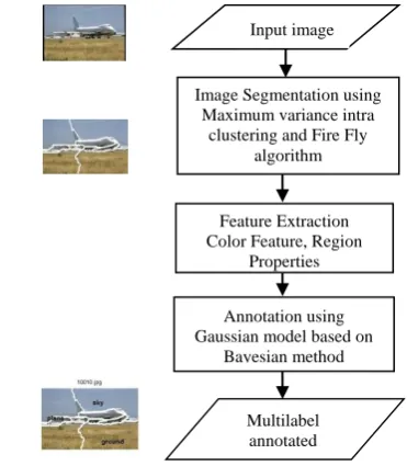
Fig. 1. The Proposed Multilabel Image Annotation System
One of the efficient methods for image segmentation is maximizing the variance Intra-cluster, which select a global threshold value by maximizing the separability of the classes in grey level images [26]. Otsu is based on maximum variance intra cluster. The basic idea of Otsu’s method is to divide the pixels into two groups at a threshold and calculate the variance between them. The bigger the variance shows the more difference between two parts. The image size is MNand the image grey level isL. The grey range is 0~L-1. The pixels number of grayscale level I
isni. Thus, the number of the image pixels is
N M n n L
i i
10 , the probability distribution is:
10
1
,
Li i i
i
p
n
n
P
(15)The image is divided into two classes with the standard threshold
t
. The class c1includes the pixel itand the class c2 includes the pixeli
t
. Cumulative probability of1
c and c2 is:
ti
p
iw
0
1 ,
11 1
2
1
L
t
i
p
iw
w
(16)Calculated mean levels:
ti 0
ip
iw
11
(
)
,
1
1 2
2 ( )
L
t
i ipi w
(17)Variance of class c1 and class c2 is:
ti 0
i
p
iw
12 1 2
1
(
)
,
1
1 2
2 2 2
2
(
)
L
t
i
i
p
iw
(18)Variance inter cluster is: 2 2 2 2 1 1
2
w
w
w
(19) Variance intra cluster is:
2 1 2 2 1 2 2 2 2 1 1 2
) ( )
( )
(
B w T w T ww (20)
The best threshold value
B
T
should satisfy the condition after the image is divided into two categories c1 and c1:]
max[
2
2
T BB
(21)When the image is segmented to more than two categories, the Otsu method should be extended to more thresholds, the equations will be as follows:
2 3 3 2 2 2 2 1 1
2
w
w
w
w
(22)2 3 3 2 2 2 2 1 1 2
) ( ) ( )
( T T T
B w w w
(23)
]
max[
2 2, 2
1
Th Th
B (24)However, with increasing the number of categories, computing rate and total runtimes also increase. Here we use modified Otsu which is a combination of the Firefly algorithm with Otsu’s method to find optimal threshold of images and increasing segmentation result accuracy [26].
B. Firefly Algorithm
The Firefly algorithm (FA) is a novel metaheuristic, which is inspired by the behaviour of fireflies [27, 28, 29]. In the Firefly algorithm, there are three idealized rules. First, all fireflies are unisex, and they will move towards more attractive and brighter ones regardless of their sex. Next, the attractiveness(r)of a firefly is proportional to its brightness which decreases as the distance from the other firefly increases. If there is not a more attractive firefly than a particular one, it will move randomly. For maximization problems, the brightness is proportional to the value of the objective function [26].
2
)
(
r
oe
r
(25) Where odenotes the maximum attractiveness (at r0) and
is the light absorption coefficient, which controls the decrease of the light intensity. The distance intra any two fireflies i and j at xi and xj, respectively, is the Cartesian distance [28].
d
k
k j k i j
i
ij x x x x
r
1
2 ,
, )
( (26)
Where xi,k is the kthcomponent of the spatial coordinate
i
x of ith firefly and d denotes the number of dimensions. The movement of a firefly i is determined by the following form [28].
)
)
2
1
(
(
)
(
2
rand
x
x
e
x
x
i i
o r j i
(27)The first term is the current position of a firefly i, the second term denotes a firefly’s attractiveness and the last
Multilabel annotated image Annotation using Gaussian model based on
Bayesian method Image Segmentation using
Maximum variance intra clustering and Fire Fly
algorithm
Feature Extraction Color Feature, Region
term is used for the random movement if there are not any brighter firefly (rand is a random number generator uniformly distributed in the range 0,1 ). For most cases
1 0
[image:5.595.326.537.588.747.2] and
0,1. In practice the light absorption coefficient γ varies from 0.1 to 10. This parameter describes the variation of the attractiveness and its value is responsible for the speed of FA convergence [28]. The flowchart of the algorithm is shown in Fig.2.Fig. 2. The Flowchart of the Maximum Variance Intracluster using Firefly algorithm
Maximum Variance Intra Cluster (Otsu) using Firefly algorithm: The pseudo code of the algorithm is:
1. Initialize algorithm’s parameters:
- Number of fireflies (n) acc.to thresholds
- α, ß and γ according to [28]
- Maximum number of generations (Max-Gen).
-Define objective function f(x) variance of segment
-Generate initial population of fireflies
-Light intensity of firefly Ii at xi is objective fn. f(xi) 2. While k < MaxGen // (k = 1: MaxGen)
For i = 1: n //all n fireflies For j = 1: n
If (Ij > Ii) move firefly i to j in acc. to Eq. (27); End if Obtain attractiveness acc. to Eq. (25) and Eq. (26) Find new solutions and update light intensity End for j
End for i
Rank the fireflies and find the current best End while
3. Find the fireflies with the highest light intensity. Image is segmented by the optimal result obtained.
C. Feature Extraction
The term feature extraction comes from pattern classification theory [29]. Its goal is twofold. Firstly, to transform the original image data into features that are more useful for classification than the original data. Secondly, reduce the computational complexity [29, 30, 31]. Some colour descriptors like correlogram, colour structure descriptor (CSV) and colour coherence vector (CVV) capture both colour and texture features. However, they are applied to entire image. Texture descriptors like edge histogram, co-occurrence matrix, directionality and spectral methods capture both texture and shape features [5].
Global features are calculated on the whole image using the moment histogram. These are mean and standard deviation. This gives 2 features. Regional Color Features: are widely used for image representation because of their simplicity and effectiveness. Colors can be represented by variable combinations of the three RGB primary color space [4, 22, 27]. However some other color spaces can be used for representing the color feature, such as HSV and Lab. A Lab color space is a color-opponent space with dimension L for lightness while a and b for the color-opponent dimensions. The Lab color space includes all perceivable colors. One of the most important attributes of the Lab model is device independence. In our work we calculate the mean
, standard deviation , and skewness
3for each channel in the Lab color space.
1
0
) ( G
i i ip
(25)
1
0 2
) ( ) (
G
i
i p
i
(26)
1
0 3 3
3 ( ) ()
G
i
i p i
(27)
Where i is a random variable indicating intensity,
) (i
p is the histogram of the intensity levels in a region and
G is the number of possible intensity levels. This yields a 9-dimensional color vector. Region properties describe the outer shape via some statistical expression. Several calculations are made using Matlab [32], which are: Area, Boundary/area and Convexity. Region properties yield 3
features. Thus the total features used are 14 features.
Fig. 3. Labeling of segmented images Y
Initialize fireflies and parameters
Calculate the variance for each segment
Better than the corresponding
fireflies
Move fireflies to new position
biggest iteration number start
Let it be the optimal threshold. Segment images with this
optimal threshold
end N
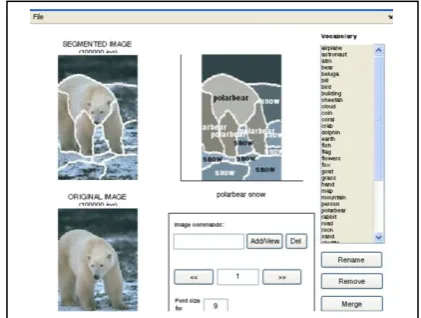
D. Labeling Segmented Images
The segmented images now consist of blobs, and each blob is labeled with word (Fig. 3). Thus we obtain a dataset of labeled images.
A. Auto annotation strategy
Annotation can be done by predicting words with high posterior probability given the image. In order to obtain the word posterior probabilities for the whole image, the word posterior probabilities of the regions in the image, provided by the probability table, are summed together. For the image
I, we can write,
L
i
i
b p I p
1 ) | ( ) |
( (28)
Fig. 4. Auto-annotation strategy. Word posterior probabilities for the regions of the image .Then the best n words with the highest probability are chosen to annotate the image
s
bi' are the blobs in the image and L is number of words in the image. Then, the sum of these word posterior probabilities is normalized to one. Fig. 4 shows an example for obtaining the word posterior probabilities for the image. In order to auto-annotate the images we predict n words with the highest probability, where n is a predefined number.
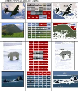
1:http://www.cs.ubc.ca/~carbo;
Fig. 5. Original images and annotated images using Grid and Modified Otsu
V. EXPERIMENTS
A. Database
[image:6.595.53.294.186.319.2] [image:6.595.42.295.450.742.2]To validate our method we use the publicly available Corel dataset, since it contains multi-label images and a variable number of objects per image. It also allows comparisons with another MIML approach and other state-of the-art methods. In the following experiments we use the Corel database (1).The database contains 2 sets, Corela and Corelb. Corela, has 200 images with 18 words in the train set. Corelb data set contains a total of 197 images with 27 words in the train set. Both sets are divided into train and test sets in the ratio 3:1. Sample of the images is shown in Fig. 5.
In our experiments, we used 3 kinds of Segmentation. In the first, we used a uniform grid of patches over the image, in the second we used the Otsu method based on the Maximum Variance Intra-Cluster as mentioned before, then finally we used the proposed modified Otsu.
The features were extracted as described before, thus obtaining 14 features. The framework provided by imagetrans1 was used extensively for building a Gaussian model [32]. For evaluation of the results several metrics are used to measure accuracy and retrieval effectiveness, the following statistics were collected: (1) Precision (p): The ratio of correctly classified instances Numcorrect to the total
number of instances classified as the class under
consideration Numretrieved. (2) Label % (label word
frequency): represents the probability of finding a particular
word in an image region; and Annotation% (annotation
word freq): represents the probability of finding a particular
word in the manually-annotated image. Results for evaluation of the image annotation are shown in Tables I to IV
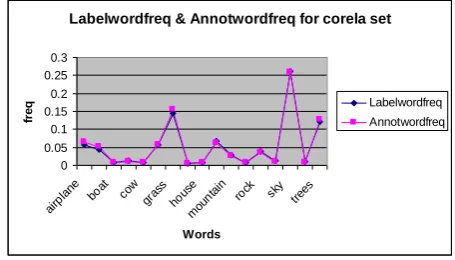
The precision of the used model averaged over the 6 trials. Precision is defined as the probability the model’s prediction is correct for a particular word and blob. Note that some words do not appear in both the training and test sets, hence the “n/a”. For Corela and Corelb sets of images, the labelword frequency and annotation word frequency are shown for the used words Fig. 6 and Fig. 7. They are roughly the same for all categories in the data set, which is a good thing and proves that the evaluation system is working right and was able to predict the label% using the annotation %.
TABLEI
RESULTS ON CORELA SET USING: OTSU
[image:6.595.335.519.609.785.2]TABLEII
RESULTS ON CORELA SET USING:MODIFIED OTSU
Using Modified Otsu Method
The precision for each individual word was also calculated for the used methods and shown in Table VII. The individual precision is defined as the probability the prediction is correct for a particular word and blob. The decrease in performance of these classes may be attributed to the small training and test images of these classes. Also the total precision was calculated. It is defined as the probability the prediction is correct for all words and all blobs. The total precision showed improvement from 0.077 to 0.109 to 0.211 for corela set and 0.120 to 0.185 to 0.235 for corelb set. The results are shown in Table V. Some objects decreased a little, but other objects improved significantly like grass, trees and water whose prediction were correct most of the time. Obviously, it is difficult problem, so it will be hard to achieve 100% accuracy. Although the individual precision may not be higher in some objects, yet the most important is the overall precision as the image is annotated with more than words not only one word.
TABLEIII
RESULTS ON CORELBSET USING: OTSU
Using Otsu Method
TABLEIV
RESULTS ON CORELBSET USING: MODIFIED OTSU
Using Modified Otsu Method
[image:7.595.313.541.394.524.2]The total precision for the modified Otsu improved significantly compared to the ordinary Otsu method, this is attributed to the segmentation technique that improved the inter-label locality. Furthermore, the features used improved the inter-label similarity. The Bayesian model applied provided better correspondence between words and segments. This illustrates the advantage of the multilabel multi-instance learner proposed.
[image:7.595.312.541.552.684.2]
Fig. 6. Labelword freq and Annotwordfreq for Corela set
Fig. 7. Labelword freq and Annotwordfreq for Corelb set
TABLEV
PRECISION USING OTSU AND MODIFIED OTSU ON COREL A AND COREL B
DATASETS
Grid
Precision
Otsu Precision
Mod Otsu Precision
Corela 0.077 0.109 0.211
Corelb 0.120 0.185 0.235
Labelwordfreq & Annotwordfreq for corela set
0 0.05 0.1 0.15 0.2 0.25 0.3
airp
lane boat cow gras
s hous
e mou
ntai n
rock sky trees
Words
fr
e
q Labelwordfreq
Annotwordfreq
Labelwordfreq & Annotwordfreq for corelb set
0 0.05 0.1 0.15 0.2 0.25
airp
lane bird cora l
fox pola
rbea r
sand snowtrack s
wat er
Words
fr
e
q Labelwordfreq
VI. DISCUSSION AND CONCLUSIONS
This study has evaluated the effectiveness of feature extraction and selection techniques applied to data using Bayesian method. The most noticeable effect is the improvement in the correctly classified instances which was affected greatly by the right choice of the segmentation technique based on the proposed Firefly algorithm and using Translation model.
The performance can be improved without much effort since most of these techniques are not time/computing intensive. This is true for any learning algorithm, since the complexity of the data used directly affects the learning algorithm's performance. Feature selection, when used along with any learning system, can help improve performance of these systems even further with minimal additional effort.
By selecting useful features from the data set, we are essentially reducing the number of features needed for these credit-risk evaluation decisions. This in turn translates to reduction in data gathering costs as well as storage and maintenance costs associated with features that are not necessarily useful for the decision problem of interest
REFERENCES
[1] Z. Zhou, M. Zhang, “Multi-instance multi-label learning with application to scene classification”, Proceedings of the International conference on Advances in Neural Information Processing Systems,
Canada, 2006, vol. 19, pp. 1609-1616.
[2] T. Sumathi, C.L. Devasena, “An overview of automated image annotation approaches,” International Journal of Research and Reviews in Information Sciences, vol. 21, pp. 1–6, 2011.
[3] J. Jeon, V. Lavrenko, R. Manmatha, “Automatic image annotation and retrieval using cross-media relevance models” , Proceedings of the 26th International ACM Conference on Research and Development
in Information Retrieval, Canada, pp. 119-126, 2004
[4] C. F. Tsai, C. Hung, “ Automatically annotating images with keywords: a review of image annotation systems”, Recent Patents on Computer Science, vol. 1, no. 1, pp. 55-68, 2008
[5] D. Zhang, M. Islam, G. Lu, “'A review on automatic image annotation techniques”, Pattern Recognition, 2012, vol. 45, no. 1, pp. 346-362 [6] G. Carnerio, N. Vasconelos, “Formulating semantic image annotation
as a supervised learning problem”, Proceedings of the IEEE Conference on Computer Vision and Pattern Recognition, San Diego, 2005, pp. 163-168
[7] V. Lavrenko, R. Manmatha, J. Jeon, “A model for learning the semantics of pictures”, Proceedings of the International Conference on Neural Information Processing Systems, Canada, 2003, pp. 553-560
[8] J. Liu, B. Wang, M. Li, et al. “Dual Cross-Media Relevance Model for Image Annotation”, Proceedings of the 15th International
Conference on Multimedia, Germany, 2007, pp. 605-614.
[9] B. K. Bao, T. Li, S. Yan, “Hidden-concept driven multi-label image annotation and label ranking”, IEEE Transactions on Multimedia, , vol. 14, no. 1, pp. 199-210, 2012.
[10] X. Xue, H. Luo, J. Fan, “Structured max-margin learning for multi-label image annotation”, Proceedings of the 9th ACM International
Conference on Image and Video Retrieval, 2010, pp. 82-88
[11] X. S. Yang, X.S. He, “Firefly Algorithm: recent advances and applications”, International journal of swam intelligence, vol. 1, pp. 36-50, 2013.
[12] A. Vailaya, M. A. T. Figueiredo, A. K. Jain, et al. “Image classification for content-based indexing”, IEEE Transactions on Image Processing, vol.10, no. 1, pp. 117-130, 2001.
[13] P. Duygulu, K. Barnard, J. D. Freitas, et al. “Object recognition as machine translation: learning a lexicon for a fixed image vocabulary”,
Proceedings of the 7th European Conference on Computer Vision,
Denmark, May 2002, pp. 97-112
[14] D. M. Blei, M. I. Jordan, “Modeling annotated data ”, Proceedings of the 26th International ACM Conference on Research and Development
in Information Retrieval, Canada, 2003, pp. 127-134
[15] L. Feng, R. Manmatha, V. Lavrenko, “ Multiple bernoulli relevance models for image and video annotation”, Proceedings of the IEEE
International Conference on Computer Vision and Pattern Recognition, USA, 2004, pp. 1002-1009.
[16] A. Yavlinsky, E. Schofield, S. Ruger, “Automated image annotation using global features and robust nonparametric density estimation”,
Proceedings of the International Conference on Image and Video Retrieval, Singapore, 2005, pp. 507-517.
[17] S. Rui, W. Jin, T. S. Chua, “A novel approach to auto image annotation based on pairwise constrained clustering and semi-naı¨ve Bayesian model”, Proceedings of the 11th International Conference on Multimedia Modeling, Australia, 2005, pp. 322-327.
[18] M. Wang, X. Zhou, T. S. Chua, “Automatic image annotation via multi-label classification”, Proceedings of the International Conference on Content-Based Image and Video Retrieval, Canada, 2008, pp. 17-26.
[19] M. Johnson, R. Cipolla, “Improved image annotation and labeling through multi-label boosting”, Proceedings of the 16th British
Machine Vision conference, British Vision Machine association, UK, 2005, pp. 1-6.
[20] S. Vaijayanarasimhan, K. Grauman, “What’s it going to cost you?: predicting effort vs informativeness for multi-label image annotations”, Proceedings of the IEEE Conference on Computer Vision and Pattern Recognition, USA, 2009, pp. 2262-2269. [21] T. sumathi, C. L. Devasena, R. Revathi, et al. “Automatic image
annotation and retrieval using multi-Instance multi-label learning”,
Bonfrig International Journal of Advances in Image Processing, vol. 1, 2011.
[22] L. Setia, H. Burkhardt, “Feature selection for automatic image annotation”, Proceedings of the 28th Symposium of the German
Association for Pattern Recognition, Germany, 2006, pp. 294–303. [23] S. Barrat, S. Tabbone, “Modeling, classifying and annotating weakly
annotated images using bayesian network”, Journal of Visual Communication Image Retrieval, vol. 21, (2), pp. 355-363, 2010. [24] R. Zhang, M. Zhang, W. Y. Ma, “A probabilistic semantic model for
image annotation and multi-modal image retrieval”, Proceedings of the 10th IEEE International Conference on Computer Vision, China, 2005, pp. 846-851.
[25] T. Hassanzadeh, H. Vojodi, M. E. Mghadam, “An image segmentation approach based on maximum variance intra-cluster method and firefly algorithm”, Proceedings of the 7th International
conference on Natural computation, China, July 2011, pp. 1817-1821, [26] X. S. Yang, “Firefly algorithm, stochastic test functions and design optimisation”, International Journal of Bio-Inspired Computation, vol. 2, no. 2, pp. 78–84, 2010.
[27] J. Kwiecien, J. B. Filipowicz, “Firefly algorithm in optimization of queueing systems”, Bulletin of the Polish Academy of Sciences Technical Sciences, vol. 60, 2012.
[28] X. S. Yang, “Firefly algorithms for multimodal optimization”,
stochastic algorithms: foundations and applications, Lecture Notes in Computer Sciences, vol. 5, pp. 169-178, 2009.
[29] S. Kuthan, D. Brown, “Extraction of attributes, nature and context of images”, International Conference of Pattern Recognition and Image Processing, Austria, 2005.
[30] W. Luo, “Comparison for edge detection of Colony Images”,
International Journal of Computer Science and Network Security, vol. 6, no. 9, pp. 211-215, 2006.
[31] R. C. Gonzalez, R. E. Woods, S. L. Eddins, “Digital Image Processing and Image Processing using MATLAB ' (Prentice Hall, 2004)
[32] P. Carbonetto, N. D. Freitas, K. Barnard, “A statistical model for general contextual object recognition”, Proceedings of the 8th European Conference on Computer Vision, Czech Republic, 2004, pp. 350-362.
[33] F. Kang, R. Jin, J. Y. Chai, “Regularizing translation models for better automatic image annotation”, Proceedings of the 13th ACM
Conference on Information and Knowledge Management, USA, 2004 [34] Z. Li, Z. Tang, Z. Li, et al. “Combining generative /discriminative
learning for automatic image annotation and retrieval”, International Journal of Intelligence Science, vol. 2, pp. 55-62, 2011.