Ferromagnetic nanoparticles with strong surface anisotropy: Spin structures and magnetisation processes

Ferromagnetic nanoparticles with strong surface anisotropy:

Spin structures and magnetization processes

L. Berger, Y. Labaye, and M. Tamine

Laboratoire de Physique de l’Etat Condensé, CNRS UMR 6087, Université du Maine, 72085 Le Mans, Cedex 9, France

J. M. D. Coey

School of Physics and CRANN, Trinity College, Dublin 2, Ireland 共Received 7 November 2007; published 24 March 2008兲

Monte Carlo simulations are used to investigate the effect of surface anisotropy on the spin configurations and hysteresis loops of ferromagnetic nanoparticles. Spherical particles of radius␳aare composed ofNatoms located on a simple cubic lattice with interatomic spacinga. The particles have 2艋␳艋13. A classical Heisen-berg model is assumed, with surface and bulk anisotropy. When surface anisotropy is positive there are two types of ground states separated by a large energy barrier: a “throttled” configuration with reduced magneti-zation for intermediate values of surface anisotropy and a “hedgehog” configuration with zero magnetimagneti-zation in the strong surface anisotropy limit. Beyond a threshold, surface anisotropy of either sign induces具111典easy axes for the net magnetization. Easy-axis hysteresis loops are then square, with a continuous approach to saturation, and the effective anisotropy is deduced either from the switching field or from the initial slope of the perpendicular magnetization curve. The hedgehog state shows a stepwise magnetization curve involving ␳ discrete configurations, and it passes to a throttled configuration before saturating. The hysteresis loop has the unusual feature that it involves a state in the first quadrant, which lies on the reversible initial magnetization curve; it is possible to recover the zero-field cooled state after saturation. A survey of the exchange and anisotropy parameters for a range of ferromagnetic materials indicates that the effects of surface anisotropy on the spin configuration should be most evident in nanoparticles of ferromagnetic actinide compounds such as US, and rare-earth metals and alloys with Curie points below room temperature; the effects in nanoparticles of 3dferromagnets and their alloys are usually insignificant, with the possible exception of FePt.

DOI:10.1103/PhysRevB.77.104431 PACS number共s兲: 75.70.Rf, 75.30.Gw, 05.10.Ln, 75.40.Mg

I. INTRODUCTION

Magnetic nanoparticles are of interest both for fundamen-tal reasons, and on account of their uses as ferrofluids, cata-lysts, and magnetic storage media. The magnetic properties of fine particles are influenced by surface effects, which be-come increasingly important as the particle size decreases. The surface effects are related to the broken symmetry of the crystal structure, whereas finite-size effects are directly at-tributed to the nanometric dimensions of the particles.

Much attention has been devoted to systems consisting of isolated nanoparticles for which experiments have indicated different magnetic properties of the surface and the bulk.1–8

The principal effects observed in ferromagnetic fine particles include the following.

共1兲Ill-defined Curie temperature, which may be reduced compared to the bulk value.

共2兲 Decreased共sometimes increased兲 saturation magneti-zationMs.

共3兲Slow approach to magnetic saturation associated with surface spin disorder.

共4兲Superparamagnetism.

共5兲Single-domain behavior. The critical single-domain ra-diusR_sd= 36␬l_exis of order 10 nm. Here␬=共K₁/␮₀M_s2兲1/2_is

the dimensionless hardness parameter andlex=共A/␮0Ms

2_兲1/2

is the exchange length which is about 2 nm for typical ferromagnets.9

共6兲Magnetization reversal by coherent rotation. The criti-cal coherence radiusRcoh=冑共24兲lex.9

共7兲An effective anisotropy constantKeffwhich may vary

asR−1whereRis the particle radius.

A feature of magnetic fine particles is surface anisotropy. The effect was first discussed by Néel,10 _{who considered a}

phenomenological magnetoelastic expression and estimated the magnitude of the anisotropy asKs⬇1 mJ m−2. This cor-responds to an anisotropy energy per surface atom ␬s=Ks␻2/3 where ␻ is the atomic volume 共⬇1.2 ⫻10−29m−3for iron兲equivalent to about 4 K, which exceeds by an order of magnitude the values of bulk anisotropy or dipole-dipole interactions in 3d magnets. In nanoparticles, with their large surface to volume ratio 共Table I兲, surface anisotropy is expected to be second only to exchange in de-termining the magnetic properties.

Previous simulations of the magnetic ground state and hysteresis in ferromagnetic nanoparticles have been based on the Landau–Lifschitz–Gilbert equation11–13 _{using a Runge–}

Kutta algorithm. The elements are shrunk to the point where they represent only a few atoms, or even a single atom,14_and

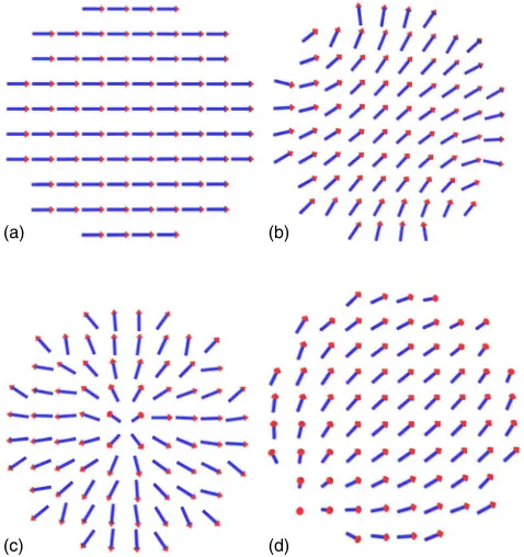
are treated as classical vectors. An alternative approach is to exploit the power of computer clusters to access the ground state and trace the field and time dependences of the spin configurations. We adopted the second approach in an earlier study of a ferromagnetic nanoparticles, where we were able to show that two types of spin structure develop in response to surface anisotropy.15_{When the value of␬}

which are normal to the surface cause the ferromagnetic con-figuration to deform into a “throttled” structure 关Fig.1共b兲兴, also sometimes known as the “flower” structure. However, beyond a critical value␬s⬇J, there is an abrupt transition to a “hedgehog” structure with no net moment关Fig.1共c兲兴.15,16

The singularity at the heart of the hedgehog is modified by dipole-dipole interactions. On the other hand, when ␬s is negative, the easy directions lie parallel to the surface, and the spins adopt an “artichoke” configuration 关Fig. 1共d兲兴. There are also reports of Monte Carlo simulations of two-dimensional magnetic nanodots with surface anisotropy.17,18

Here the focus is on three-dimensional particles with posi-tive␬s. We investigate the magnetization processes and hys-teresis for the throttled and hedgehog states. We examine the size dependence of the coercivity and consider the problem of evaluating the surface anisotropy from data on nanopar-ticle systems. Then we investigate the energy barriers be-tween different spin states by simulating the magnetic relax-ation. Finally, we review the magnitude of exchange, surface, and bulk anisotropy for a range of ferromagnetic materials, and suggest where to look for some of the predicted effects.

II. METHODS

Our model system is a spherical nanoparticle composed of atoms forming a simple cubic lattice with interatomic spac-inga. The radiusR=␳ais varied from␳= 2 to␳= 13, corre-sponding in practice to particles smaller than about 5 nm. It is important to emphasize, as illustrated in Fig. 1, that the center of the spherical particle is not located on an atomic site, but at the centroid of the eight central atoms. Each mag-netic site hasZ= 6 nearest neighbors in the volume and 3, 4, or 5 at the surface; the missing neighbors lead to the surface anisotropy. The sphere contains N atoms with Ns of them located on the surface. Values ofNandNs, and the numbers of atoms with different coordinations are listed in TableI. A typical particle with␳= 5 is illustrated in Fig.2.

A vector spin 兩S兩= 1 is associated with each atom. The system is described by a classical Heisenberg Hamiltonian, which includes terms denoting the nearest-neighbor ex-change interaction, the anisotropy energy, the dipole interac-tion, and the Zeeman energy. For a given site i it may be expressed as

Hi= −⌺j=1 6

JSi·Sj−␬i共Si·ni兲2−␮i共Bdip+B兲·Si, 共1兲

where the sum is over the j nearest neighbors.J is the ex-change coupling constant, Si andSj are the spins on sitesi andj, and␬iis the anisotropy constant, taken as␬vfor all the sites with six nearest neighbors, or as␬sfor the sites belong-ing to the surface. We take the bulk anisotropy ␬v to be uniaxial along theOzaxis. The surface anisotropy direction is defined as

7 168 144 144 1016 5.36 456 1472 0.31

8 248 120 264 1544 5.43 632 2176 0.29

9 240 264 288 2320 5.51 792 3112 0.25

10 320 288 360 3256 5.55 968 4224 0.23

11 408 288 504 4416 5.59 1200 5616 0.21

12 408 456 552 5792 5.63 1416 7208 0.20

13 560 432 696 7640 5.65 1688 9328 0.18

(a)

(c)

(b)

(d)

␴i=⌺jrij/兩⌺jrij兩. 共2兲

These directions are 具111典 for sites with Z= 3, 具110典 for Z

= 4, and具100典for Z= 5. They lie close to the surface normal at every site.Bdipis the dipole field,Bis the external applied

field, and␮iis the atomic magnetic moment in Bohr magne-tons. For convenience in our simulation, we setJ= 1000共 fer-romagnetic coupling兲 and choose ␬v= 0, 10, or 50 and ␬s = 1 – 1200. Having set the value ofJ, all the other interactions can be normalized to the exchange. When passing from the single-site Hamiltonian共1兲to the Hamiltonian for the whole system, factors of 1/2 appear in the exchange and dipole terms to avoid double counting. Noting that the maximum value of the dipole interaction for the particles studied does not exceed unity, we neglect this term in the following cal-culations.

The simulations have been performed in three steps: 共i兲 First we analyze, as a function of particle size ␳, the spin structure and magnetization of the ground state, which is strongly dependent on surface anisotropy␬s.共ii兲The second step is to describe the initial magnetization curves and hys-teresis loops for particles with a particular spin configuration and a chosen value of ␬s. 共iii兲 Finally, the energy barriers separating hedgehog and throttled configurations are de-duced from the Monte Carlo simulations, and analyzed as a function of the applied field.

All the simulations were performed on a Beowulf-class cluster composed of 35 PCs with dual Pentium III 600 MHz processors.19 _{Starting from a random spin configuration at}

high temperature, the energy is minimized by simulated an-nealing using the Metropolis algorithm with a decreasing exponential law for temperatureT␥with␥= 0.985. We used unrestricted classical angular dynamics 关the spin directions 共␪,␾兲are chosen randomly兴. The simulations were started at

T= 2000, well above TC. The final temperature is normally ⬍1. The number of Monte Carlo steps per spin was 104_{. The}

time to reach the local equilibrium state for typical simula-tions was 1 – 100 h, depending on particle size.

For an extended simple cubic lattice the relation between exchange and Curie temperatureTCis20

TC= 1.44JS2. 共3兲

HenceJ= 1000 givesTC= 1440. This is approximatelyTCfor Co.

III. RESULTS

A. Ground state configuration

We first determine the magnetic phase diagram as a func-tion of particle radius␳ withN⬇4/3␲␳3 _{atoms in the}

par-ticle andNs⬇4␲␳2 of them are lying on surface where they have surface anisotropy␬s. The volume anisotropy␬vis var-ied 共0, 10, 50兲, while keeping the exchange coupling J

= 1000. Energies of the hedgehog and throttled states are evaluated, and the lower energy state is the stable one. En-ergies calculated from the Monte Carlo simulation are com-pared to those of an approximate analytical calculation, de-scribed below. Results are presented in Fig.3.

The energy of the hedgehog configuration can be evalu-ated approximately, assuming that the magnetic momentSiat sitei is given by ri/兩ri兩. Surface anisotropy energy Es, vol-ume anisotropy energy Ev, and exchange energy Eex are

given, respectively, by −4␲␳2_␬

s, −4␲␳2共␳/3 − 1兲␬v/3, and −共2/3␲␳3_{具Z典J兲兵1 + 3 arctan共2␳兲/共4␳}3_{兲− 3/共2␳}2_{兲其, where 具Z典}

is the average number of nearest neighbors which is listed in Table I. The exchange term is obtained by considering the interaction of a pair of neighboring spins at a distance␦from the center of the particle,Jcos兵2 arctan关1/共2␦兲兴其. Integrating over spherical shells which contain 4␲␦2_{d␦such spins gives}

the expression for the exchange energy. As far as we know, no analytical expression exists forSiin the throttled configu-ration, so we base an approximate analysis on a uniaxial ferromagnetic configuration 关Fig. 1共a兲兴. In this case Si=ez, where ez is the unit vector in the z direction. The surface anisotropy, volume anisotropy, and exchange energies are FIG. 2. 共Color online兲A particle with radius␳= 5. 43% of the

atoms lies at the surface. Those with 3, 4, and 5 neighbors are colored green共light gray兲, dark blue共dark gray兲, red共medium light gray兲, and inner atoms are white.

−4␲2_␳2_{␬s/3, −4␲␳}2_{共␳/3 − 1兲␬v, and −2/3␲␳}3_具Z典J,

respec-tively. The phase boundary versus radius for given values of

␬v and Jis obtained by equating the sum of these energies

E=Es+Ev+Eexfor each configuration. This leads to

␬s=␬v共␳/3 − 1兲− 3具Z典J/4关arctan共2␳兲/共4␳2兲− 1/共2␳兲兴. 共4兲 To better approximate the throttled energy configuration, we need to reduce the surface anisotropy energy of the uniaxial configuration. This is done with a configuration which has a uniaxial ferromagnetic core and a surface with radially ori-ented spins. The expression for␬sthen becomes

␬s=关2共␳/3 − 1兲␬v/3

−具Z典J/2兵arctan共2␳兲/共4␳2_{兲− 1/共2␳兲其兴/共2/3 −␣兲, 共5兲}

with␣ ranging from 0 for the uniaxial configuration to 2/3 for radial spins on the surface. The ␬s共␳兲 curves obtained from Eq.共5兲with ␣= 0.4 are similar to those of the Monte Carlo simulations. The discrepancy between curves is cer-tainly due to the approximation involved in assuming a quasiuniaxial configuration instead of the true throttled con-figuration.

The energy difference between the throttled and hedgehog states in the phase diagram of Fig. 3 is remarkably small. The dominant energy is the exchange, which is roughly −具Z典J/2 or⬇2500 per site. Figure 4 shows the energy per site ␧=E/N as a function of ␬s for the ␳= 5 particle. The crossover occurs at ␬s⬇800. To obtain the curves, ␬s was varied in the course of the simulation. At␬s= 0 the energy difference is about 100, or 4% of the exchange energy.

The hedgehog state is obviously twofold degenerate, in the sense thatSi→−Si gives an inverted hedgehog with the same energy. In small particles, there is no continuous rota-tion symmetry on account of the stepped nature of the par-ticle surface, which has the symmetry of a cube.

The throttled state is also twofold degenerate in the sense that Si→−Si gives a throttled state with the same energy. Since there is a net moment, there should be an easy axis. Our simulations, carried out in this case by cooling from temperature 2000 to 0.15, show clearly the existence of具111典

easy axes when␬s⬎450. A convenient way to represent the easy axis ␴ is to take the scalar product ⌸ of ␴ with 共1/冑3兲关⫾1 ,⫾1 ,⫾1兴in such a way that each component of the scalar product is positive. This gives⌸= 1 for具111典,⌸ = 2/冑6共0.82兲for具110典, and⌸= 1/冑3共0.58兲for具100典. From Fig. 5 it is evident that a 具111典 direction is easy when ␬s ⬎450, but the orientation appears to be random for smaller values of␬s. This is probably because the base temperature of the simulations is higher than the effective anisotropy per site␬_eff.

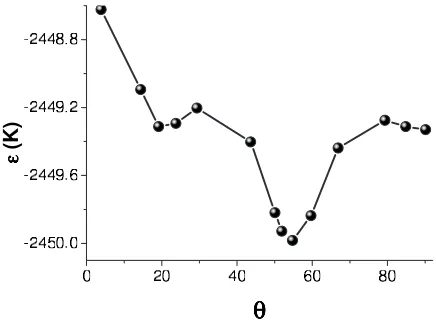
Easy axes arise wherever the surface anisotropy is able to deform the collinear ferromagnetic structure. The easy direc-tion was also determined by fixing the direcdirec-tion of magneti-zation of a nucleus of eight atoms at the center of the particle and then carrying out a Monte Carlo simulation, cooling fromT= 2000, down toT= 0.15. The energy is minimum for a 具111典 direction 共i.e., ␪= 54.7°兲, as shown in Fig. 6. The average anisotropy energy per site for the particle with ␳ = 5 and␬s= 500 is only 1.4.

Finally, we mention the case␬s⬍0, which corresponds to easy-plane anisotropy of the surface sites. The effect of the FIG. 4. Energy difference between the throttled and hedgehog

states for a particle with radius␳= 5. Error bars are smaller than the

plot symbols. FIG. 5. Results of multiple Monte Carlo simulations to

deter-mine the easy axis of a particle with radius␳= 5.具111典is easy when surface anisotropy␬s⬎450.⌸is defined in the text.

planar anisotropy is to induce an artichokelike spin structure, where the surface spins tend to lie parallel to the surface. Increasing the value of兩␬s兩leads to a continuous deformation of the ferromagnetic state. The easy axis is again具111典.

B. Hysteresis loops

Next we study the virgin magnetization curve and the complete hysteresis loop for particles withJ= 1000 and val-ues of ␬s which give either a throttled or a hedgehog con-figuration. For smaller values of␬s the rotation is coherent, and the nanoparticles behave like macrospins, as in the Stoner–Wohlfarth model.21–24 _{From the ground state, the}

magnetic field is increased in constant steps and the energy is minimized at each step using 80 000 Monte Carlo iterations, after rejecting the first 10 000 to allow for the approach to thermal equilibrium. The hysteresis is traced out by increas-ing the magnetic field B from zero up to B_max 共60⬍B_max

⬍500兲, then reducing it to −Bmaxand again increasingBmax

in order to describe a complete loop. The moment␮ in Eq. 共1兲is taken as unity, soBcorresponds to the field in units of

kB/␮B⬇1.5 T. In one case共␳= 5,␬s= 1050,␬v= 10兲this pro-cess was repeated ten times to be sure of the reproducibility of the results. In addition, minor loops have been investi-gated, where the maximum field is less thanBmax.

1. Throttled configuration

Here we choose ␬s= 400– 800 and ␬v= 0, and apply the magnetic field along a关111兴easy direction. There is there-fore already a large moment in the virgin state. Particle ra-dius is varied from ␳= 2 to ␳= 13. The hysteresis loops shown in Fig.7are for␬s= 400. The switching fieldBsvaries

irregularly and nonmonotonically with particle radius. The effective anisotropy constant deduced from the anisotropy field by the Stoner–Wohlfarth relationBa= 2␬eff/␮is plotted

in Fig.8. Again we take␮= 1.

An alternative method to evaluate the effective anisotropy is to apply a small magnetic field perpendicular to the easy direction, and to determine the slope of the initial magneti-zation curve共Fig.9兲. The first step in the perpendicular mag-netization curves corresponds to switching to the具111典easy axis closest to the applied field direction. The second step corresponds to complete alignment with the applied field. Extrapolation of the initial curve to the spontaneous magne-tizationmsof the particle gives the anisotropy fieldBawhich is also related to the effective anisotropy ␬_eff by ␬_eff =Bams/2. The two independent methods of determining ␬eff

FIG. 7. Hysteresis loops simu-lated with the applied field along the 关111兴 direction for particles with surface anisotropy ␬s= 400 and different radii␳. When error bars are not shown, they are smaller than the plot symbols.

are in rather good agreement, and the irregular variation with particle size in Fig.8 is not an artifact. It is noteworthy that the values of␬_effare more than an order of magnitude less than␬seven though 20%–75% of the atoms in the particles with 2ⱕ␳ⱕ12 are surface atoms. This is because the

aniso-center of symmetry of the magnetic moment distribution of one interatomic distance in the direction opposite to the field 关Figs.10共a兲–10共d兲兴. It is interesting that this part of the mag-netization curve is fully reversible, and the original hedgehog state can be recovered by reducing the field to zero. How-ever, at a critical value of applied field共point d in Fig.10兲, there is a jump to a throttled configuration, and the magne-tization process becomes irreversible. On reducingBto zero from point e in Fig.10, the nanosphere remains in a throttled configuration, which is a metastable state in low fields, where the hedgehog energy is actually lower.

The virgin magnetization curve is reached again at point l in the first quadrant in Fig.10, after magnetization reversal and increasing the magnetic field in the reverse direction. Remarkably, the displaced hedgehog configuration of Fig. 10共d兲is found again, and on reducingBto zero from point l FIG. 9. Magnetization curve obtained when the field is applied

perpendicular to the具111典easy axis for a particle with radius␳= 5 and surface anisotropy ␬s= 400 having a throttled spin configura-tion. Anisotropy fieldBamay be deduced from the initial slope, as described in the text.

it is possible to recover the initial hedgehog state with zero magnetization. It is the nucleation of the group of four inward-pointing spins in Fig.10共h兲that decides the inward-pointing hedgehog. This recovery of reversible behavior after saturation is a most unusual effect of the strong surface an-isotropy of these nanoparticles. It is only in such nanopar-ticles that the major loop can rejoin the initial curve.

C. Energy barriers and magnetic relaxation

Although the energies of the throttled and hedgehog con-figurations are very similar, the existence of broad hysteresis loops suggests that the barriers separating the two configu-rations are greater than their difference in energy. The ener-gies of the two configurations involved in the hysteresis loop of Fig.10are shown in Fig.11.

Thermal fluctuations of the magnetic moment of a single-domain ferromagnetic particle and its approach to equilib-rium are well described by Néel–Brown model.24,25 _The

main assumptions in this model are that the magnetization is uniform and the anisotropy is uniaxial so that the relaxation can be described by a single relaxation time␶. In the case of an isolated nanoparticle, the magnetic relaxation is given by an Arrhenius law of the form

␶=␶0exp共⌬E/kBT兲, 共6兲 where␶0 is of order 10−9– 10−11s and depends weakly on

temperature, ⌬E denotes the energy barrier separating the two configurations,kBis Boltzmann’s constant, andTis tem-perature. This model is widely used to describe the time dependence of magnetization of multiparticle assemblies where a logarithmic time dependence is found—for example, in␥Fe2O3,26Ni, Co, and Dy.27This logarithmic time

depen-dence arises from a broad distribution of relaxation times␶ for the particles of different sizes.

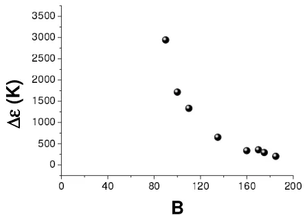
Our objective here is to give a measure of the energy barrier⌬E. Considering the relaxation from the hedgehog to the throttled configuration in a magnetic field close to that needed to make the jump d→e in Fig. 10, we performed 10 000 runs in a fixed field in the range 80–185 and at a fixed

temperature in the range 400–650. For each run, the switch-ing time␶for a single particle is recorded in units of Monte Carlo steps. Some typical data are shown in Fig.12. They are fitted to give the average value具␶典. The slope of the plot of ln具␶典vs 1/Tgives the energy barrier⌬E, and the variation of ⌬E with field B is shown in Fig. 13 for a particle with ␬s = 1100, ␬v= 10, and ␳= 5. The extrapolation of the energy barrier to zero field gives a barrier between the throttled and hedgehog configurations which is several times their energy difference. The result is reasonable and it justifies our obser-vation that the Monte Carlo simulations find the local energy minima, which are a source of hysteresis.

When a sample contains particles with a distribution of particle size and shape, the abrupt variations seen in Fig.8 are washed out. Assuming a log-normal distribution of size, the results for effective anisotropy as a function of average particle size shown in Fig.14are obtained.

FIG. 11. Energies of the states traced out in the hysteresis loop in Fig.10. The energy barrier for the transition d→e is also shown. Error bars are smaller than the plot symbols.

0 2000 4000 6000 8000

0 200 400 600 800 1000

N

(MCS)

FIG. 12. Probability distribution for the switching time for a particle with radius␳= 5 surface anisotropy␬s= 1100, uniaxial vol-ume anisotropy␬v= 10, applied fieldB= 185, andT= 350 K.

IV. DISCUSSION

A. Evaluation of surface anisotropy

It is a common practice in the literature to evaluate the effective anisotropy constant of ferromagnetic thin films and nanoparticles from a formula such as

K_eff=K_v+␩Ks, 共7兲

where␩ is an inverse length. For a film of thicknesst共two surfaces兲␩= 2/t,28_{but for a nanosphere共following Bodkeret} al.2_{兲it is taken as 3/R, where K}

effandKvhave units J m−3,

whereasKshas units J m−2. The basis of this formula is that the nanosphere contains 共4/3兲␲R3/a3 atoms, 4␲R2/a2 of which lie on the surface. If all the atoms contribute ␬v =Kva3to the anisotropy of the particle, and the surface atoms

make an additional contribution of␬s=Ksa2, the total aniso-tropy is共4/3兲␲共R/a兲3␬v+ 4␲共R/a兲2␬s, and the effective an-isotropy constant is therefore␬eff=␬v+共3/R兲␬s.

This analysis is based on the implausible assumption that the anisotropy axes in the bulk and at the surface are all parallel. In fact, we have been supposing that the surface atoms have their easy directions roughly normal to the sur-face. In the limit of a large spherical particle with a uniform density of surface atoms and radial surface anisotropy ␬s ⰆJ, so that the surface anisotropy does not modify the col-linear ferromagnetic spin alignment, the contribution of␬sto

␬effis precisely zero. On account of their underlying crystal

structure, small particles do not present a uniform density of surface atoms, as is illustrated in Fig.2for the particle with

␳= 5. The anisotropy energy has been calculated for our simple cubic particles from␳= 2 up to ␳= 13, and we con-clude that具111典are usually the easy axes, in agreement with the analysis of Garanin and Kachkachi,29 _{provided the}

sur-face anisotropy is sufficient to deform the collinear ferro-magnetic structure. These authors found that 具111典axes are easy, regardless of the sign of the surface anisotropy in the Néel model.

From the plot of our size-averaged data for␬s= 500 as a function of 1/␳ in Fig.14, we find that the slope is not 3␬s = 1500 but it is very much smaller. The procedure for

deter-mining␬sfrom␬efftherefore underestimates its value by an

order of magnitude. More serious is the absence of any com-pelling indication of a trend indicating a 1/␳ variation. It is the specific surface structure of a nanoparticle that deter-mines␬eff, not simply its radius.

B. Other models of surface anisotropy

We have chosen an algorithm for defining surface aniso-tropy, which places the local anisotropy axes roughly normal to the surface and assumes easy-axis anisotropy. The effect of the algorithm is similar to radially directed anisotropy, transverse to the surface.30 _{The original Néel}10 _{model was}

somewhat different. Néel assumed that the contribution of each nearest neighbor isE=l/2 cos2_{␪ where␪ is the angle}

between the direction of the local magnetization and the bond with the neighboring atom. His model gives the follow-ing results ifl, which is the product of magnetostriction and elastic constants, is positive: for a surface perpendicular to 具111典 there is no easy axis, for a surface perpendicular to 具100典the easy axis is具100典, and for a surface perpendicular to关011兴,关101兴, or关110兴there is an easy plane perpendicular tox,y, and z, respectively, as shown in Fig.15.

C. Comparison with real ferromagnets

The surface atoms have reduced symmetry where the axis of the electric field gradient 共the leading crystal field term

A₂0兲tends to lie perpendicular to the surface. In principle, this can lead to anisotropy which is perpendicular to the surface, or else lies in a plane parallel to the surface, depending on the sign of the crystal-field interaction. In the parallel case, other crystal-field terms such as A₂2 will determine an easy direction in the plane. We therefore anticipate that among the rare earths, atoms with a positive quadrupole moment共Sm, Er, Tm, and Yb兲 will show perpendicular-to-surface aniso-tropy, and those with a negative quadrupole moment共Pr, Nd, Tb, Dy, and Ho兲will show a parallel-to-surface anisotropy. Among the 3datoms, similar arguments suggest that Co may show perpendicular anisotropy in a crystal field where the FIG. 14. Variation of␬eff, the average anisotropy per site, for

surface anisotropy␬s= 500, uniaxial volume anisotropy␬v= 0, and a log-normal distribution of particle size.

anisotropy of Fe is parallel, but another factor intervenes in the case of these metals, namely, the orbital moment associ-ated with 3d band electrons. Here the symmetry of the face, which allows orbits to develop in the plane of the sur-face, but not in the perpendicular direction, suggests that the anisotropy due to spin-orbit coupling will inevitably be per-pendicular to the surface.31 _{The magnetization of thin films}

indicates that surface anisotropy is usually perpendicular to the surface.32

It is important to relate the physical parametersJ,␬v, and

␬s used in the Monte Carlo simulations to the values that characterize real materials. The numbers for a given simula-tion can all be scaled by a constant factor, without changing the magnetic ground state.

For the exchange, the bulk Curie temperature is used to determineJ, using Eq.共3兲. With our definition of the Heisen-berg Hamiltonian 关Eq. 共1兲, which differs by a factor of 2 from another common definition兴, Monte Carlo simulations with classical spins represented by S= 1 give kBTC/ZJ = 0.24. WithZ= 6, . Values ofJ in Kelvin for a selection of ferromagnetic materials are listed in TableII.

For the bulk anisotropy, the measured uniaxial anisotropy constantK₁共orK₁c for cubic materials兲is converted to␬vin units of Kelvin by multiplying by the volumevper magnetic ion, and dividing by Boltzmann’s constantkB.

The surface anisotropy is trickier to estimate. Evaluations based on Eq.共4兲 will tend to underestimate␬s for nanopar-ticles by as much as an order of magnitude for the reasons discussed in Sec. IV A. For cobalt, as an example, estimates from studies of nanoparticles have given values of ␬s in the range 0.2– 0.9 mJ m−3_,5 _{which correspond to ␬}

s = 0.7– 3.2 K, whereas studies of ultrathin films give values of the surface anisotropy of order 0.7 mJ m−2 _which

corre-sponds to␬s= 2.5 K.33Another approach is to take the bulk anisotropy in the most anisotropic cobalt-based alloys as a lower limit on the surface anisotropy. For example, CoPt and YCo₅haveK₁= 4.9 and 6.5 MJ m−3_{, respectively, which}

cor-respond to values of␬sof at least 9.8 or 7.9 K. Much larger anisotropy,␬s= 100 K, is reported for a single cobalt atom on Pt.34_{However, in any case, it is clear that cobalt and}

cobalt-rich alloys with their high TC values lie far below the throttled and/or hedgehog boundary at␬s/J⬇1. The value of

␬s/J is such that surface anisotropy will not significantly perturb the collinear ferromagnetic ground state. A similar expectation applies to FePt. AlthoughTC is lower than it is

for Co共TableII兲, the value ofJ= 520 K is still much greater than the bulk anisotropy␬v= 13.4 K, which is a lower limit on␬s. Even if the ratio of surface to bulk anisotropy is simi-lar to that in cobalt, we are in the region␬s/J⬇0.5 共Table II兲,35 _{where the ferromagnetic saturation is reduced by only}

about 10% by the throttled spin configuration.

The interesting effects we have found in our Monte Carlo simulations when␬s/J⬇1 are most likely to be manifest in compounds with strong surface anisotropy and weak ex-change. The best candidates are rare-earth metals and alloys, and also some actinide-based ferromagnetic compounds. Er-bium, for example, has a magnetic ordering temperature of 85 K, which corresponds toJ= 57 K, and the anisotropy con-stantK1= 7 MJ m−3 corresponds to ␬v= 15.4 K. For the rare

earths,ab initiocalculations36_{suggest that the surface}

aniso-tropy is approximately twice as large as the bulk value; hence, for Er we expect that ␬s⬇100 K. Erbium nanopar-ticles should therefore adopt a hedgehog state. Terbium, however, has TC= 221 K, which corresponds to J= 124 K, and the hard-axis anisotropy constant K1= −56 MJ m−3

cor-responds to␬v= −130 K. The surface anisotropy expected is

␬s= −1000 K.36Since the surface anisotropy is negative, and considerably larger than the exchange, it will lead to an ar-tichoke configuration like that of Fig.1共d兲.

More extreme examples with huge positive anisotropy are provided by TmNi₅, where the exchange is weak, and by US, where the uranium anisotropy is exceptionally strong, as seen in TableII. A factor of 2 is used to estimate the surface anisotropy of the actinide, by analogy with the rare earths. Both these materials can be expected to exhibit hedgehog configurations.

V. CONCLUSION

Atomic-scale Monte Carlo simulations with classical spins indicate that significant modifications of the collinear ferromagnetic spin configuration can be expected in certain ferromagnetic nanoparticles due to surface anisotropy. There are interesting steps in the hysteresis loops, which resemble those found in larger nanoparticles,37,38 _{in molecular}

magnets,39,40 _{or in rare-earth alloy thin films,}41 _{but which}

have a quite different physical explanation. In these small particles it is possible to associate the steps on the hysteresis loop with jumps between identifiable spin configurations. The reversibility of the steps in the first quadrant, after de-TABLE II. Typical values of physical parameters for selected ferromagnetic materials.

va_共nm3_{兲 T}

c共K兲 J共K兲 K1b共MJ m−3兲 ␬v共K兲 Ks共mJ m−2兲 ␬s共K兲

Co 0.011 1390 959 0.5 0.4 ⬇1 4

YCo5 0.017 987 684 6.5 7.9 ⬃20 95

FePt 0.028 750 520 6.6 13.4 ⬃34 227

Er 0.031 85 57 7 15.4 14 100

Tb 0.031 221 153 −56 −130 −140 −1000

TmNi5 0.085 4.5 3 70 300 55 774

US 0.041 177 162 1000 3000 428 6000

a_{Volume per magnetic atom.}

netic elements and their alloys usually have ␬s/JⰆ1, and their spin configurations are barely modified by surface an-isotropy. FePt is a case, however, where some measurable reduction in saturation magnetization due to a throttled spin

processor, Beowulf-class, homemade parallel computer at LPEC共website: http://weblotus.univ-lemans.fr/w3lotus兲. We are grateful to Ralph Skomski for drawing to our attention the huge anisotropy of US.

1_{S. Sun, C. B. Murray, D. Weller, L. Folks, and A. Moser, Science}

287, 1989共2000兲.

2_{F. Bodker, S. Morup, and S. Linderoth, Phys. Rev. Lett. 72, 282} 共1994兲.

3_{C. Chen, O. Kitakami, and Y. Shimada, J. Appl. Phys. 84, 2184} 共1998兲.

4_{F. Gazeau, J. C. Bacri, F. Gendron, R. Perzynski, Y. L. Raikher, V.}

I. Stephanov, and E. Dubois, J. Magn. Magn. Mater. 186, 175 共1998兲.

5_{M. Respaud, J. M. Broto, H. Rakoto, A. R. Fert, L. Thomas, B.}

Barbara, M. Verelst, E. Snoeck, P. Lecante, A. Mosset, J. Osuna, T. Ould Ely, C. Amiens, and B. Chaudret, Phys. Rev. B 57, 2925共1998兲.

6_{A. Punnoose, H. Magnone, M. S. Seehra, and J. Bonevich, Phys.}

Rev. B 64, 174420共2001兲.

7_{E. De Biasi, C. A. Ramos, R. D. Zysler, and H. Romero, Phys.}

Rev. B 65, 144416共2002兲.

8_{B. Barbara, Solid State Sci. 7, 668共2005兲.} 9_{L. Néel, Ann. Geophys.共C.N.R.S.兲 5, 99共1949兲.} 10_{L. Néel, J. Phys. Radium 15, 255共1954兲.}

11_{D. A. Dimitrov and G. M. Wysin, Phys. Rev. B 50, 3077共1994兲.} 12_{D. A. Dimitrov and G. M. Wysin, Phys. Rev. B51, 11947共1995兲.} 13_{H. Kachkachi and M. Dimian, Phys. Rev. B 66, 174419共2002兲.} 14_{M. Dimian and H. Kachkachi, J. Appl. Phys. 91, 7625共2002兲.}

15_{Y. Labaye, O. Crisan, L. Berger, J. M. Greneche, and J. M. D.}

Coey, J. Appl. Phys. 91, 8715共2002兲.

16_{O. Iglesias and A. Labarta, J. Magn. Magn. Mater. 290–291, 738} 共2005兲.

17_{V. E. Kireev and B. A. Ivanov, Phys. Rev. B 68, 104428共2003兲.}

18_{S. A. Leonel, I. A. Marques, P. Z. Coura, and B. V. Costa, J. Appl.}

Phys. 102, 104311共2007兲.

19_{F. Calvayrac, Y. Labaye, and J. C. Gimel, Tech. Sci. Inform. 21,}

1371共2002兲.

20_{P. Peczak, A. M. Ferrenberg, and D. P. Landau, Phys. Rev. B 43,}

6087共1991兲.

21_{H. Kachkachi and E. Bonet, Phys. Rev. B 73, 224402共2006兲.} 22_{J. Mazo-Zuluaga, J. Restrepo, and J. Mejia-Lopez, Physica B}

398, 187共2007兲.

23_{H. Kachkachi and H. Mahboub, J. Magn. Magn. Mater. 316, 248} 共2007兲.

24_{J. Restrepo, Y. Labaye, and J. M. Greneche, Physica B 384, 221} 共2006兲.

25_{W. F. Brown, Phys. Rev. 130, 1677共1963兲.}

26_{R. Prozorov, Y. Yeshurun, T. Prozorov, and A. Gedanken, Phys.}

Rev. B 59, 6956共1999兲.

27_{W. Wernsdorfer, E. Bonet Orozco, K. Hasselbach, A. Benoit, B.}

Barbara, N. Demoncy, A. Loiseau, H. Pascard, and D. Mailly, Phys. Rev. Lett. 78, 1791共1997兲.

28_{H. J. G. Draaisma, W. J. M. de Jonge, and F. J. A. den Broeder, J.}

Magn. Magn. Mater. 66, 351共1987兲.

29_{D. A. Garanin and H. Kachkachi, Phys. Rev. Lett. 90, 065504} 共2003兲.

30_{H. Kachkachi and H. Mahboub, J. Magn. Magn. Mater. 278, 334} 共2004兲.

31_{R. Skomski and J. M. D. Coey,Permanent Magnetism共Institute} of Physics, Bristol, 1999兲.

32_{R O’Handley, Magnetism and Magnetic Materials共Wiley, New} York, 2001兲.

33_{D. Weller, J. Stöhr, R. Nakajima, A. Carl, M. G. Samant, C.}

Chappert, R. Mégy, P. Beauvillain, P. Veillet, and G. A. Held, Phys. Rev. Lett. 75, 3752共1995兲.

34_{P. Gambardella, S. Rusponi, M. Veronese, S. S. Dhesi, C.}

Grazioli, A. Dallmeyer, I. Cabria, R. Zeller, P. H. Dederichs, K. Kern, C. Carbone, and H. Brune, Science 300, 1130共2003兲. 35_{In our earlier paper, Ref.14, we suggested that FePt nanoparticles}

may have a throttled spin structure, but there we omitted a factor 2 in the exchange, and were probably overgenerous in our esti-mate of␬s.

36_{F. Welsch, M. Fähnle, and P. J. Jensen, J. Phys.: Condens. Matter}

17, 2061共2005兲.

37_{W. Wendorsfer, K. Hasselbach, D. Mailly, B. Barbara, A. Benoit,}

L. Thomas, and G. Suran, J. Magn. Magn. Mater. 145, 33 共1995兲.

38_{S. J. Hefferman, J. N. Chapman, and S. McVitie, J. Magn. Magn.}

Mater. 95, 76,共1991兲.

39_{Jonathan R. Friedman, M. P. Sarachik, J. Tejada, and R. Ziolo,}

Phys. Rev. Lett. 76, 3830共1996兲.

40_{D. Gatteschi and R. Sessoli, J. Magn. Magn. Mater. 272–276,}

1030共2004兲.

41_{J. M. D. Coey, T. R. McGuire, and B. Tissier, Phys. Rev. B 24,}

1261共1981兲.

42_{W. Scholz, D. Suess, T. Schrefl, and J. Fidler, J. Appl. Phys. 95,}

6807共2004兲.