Inferences for Burr-X Model Based on Uniﬁed Hybrid Censored Data

(1)

Inferences for Burr-X Model Based on Unified

Hybrid Censored Data

Abdalla Rabie and Junping Li

Abstract—In this paper, Burr-X distribution with unified hybrid censored data is considered. The maximum likelihood method, the Bayesian and the E-Bayesian (the expectation of the Bayesian estimate) approaches are studied for the distribution parameter and the associated reliability function. The Bayesian and the E-Bayesian estimates are derived under LINEX and squared error loss (SEL) functions. We apply Markov chain Monte Carlo (MCMC) techniques to derive the Bayesian and the E-Bayesian estimates. Also, confidence intervals (CIs) of the maximum likelihood estimates, as well as credible intervals (CRIs) of the Bayesian and the E-Bayesian estimates, are computed. On the other hand, an example of a real data set is provided for the purpose of illustration. Finally, a numerical comparison among the proposed methods is performed.

Index Terms—Bayesian estimation, Burr-X distribution, E-Bayesian estimation, Unified hybrid censoring scheme, Maxi-mum likelihood estimation, MCMC method.

I. INTRODUCTION

G

ENERALIZED Type-I and Type-II hybrid censoring schemes (HCSs) are proposed by [1] to overcome the drawbacks of Type-I and Type-II HCSs, for more details about HCSs, one can refer to [2]. The generalized HSCs are an extension of Type-I and Type-II HCSs, therefore, we can notice two types of censoring schemes are described as follows. Generalized Type-I HCS: fix integers r, k ∈ {1,2,· · ·, n} such that k < r < n, and time T ∈(0,∞). The experiment is terminated at min{Xr:n, T}, if the k-th failure occurs before time T. If the k-th failure occurs after timeT, the experiment is terminated atXk:n.

Generalized Type-II HCS: fix integer r ∈ {1,2,· · · , n}

and time points T1, T2 ∈ (0,∞) such that T1 < T2. The

experiment is terminated at T1, if the r-th failure occurs

before time T1. If the r-th failure occurs between T1 and T2, the experiment is terminated atXr:n. Finally, if ther-th

failure occurs after time T2, the experiment is terminated at T2.

Unified HCS (UHCS) is defined by [3] as a mixture of generalized Type-I HCS and generalized Type-II HCS which can be described as follows. Suppose n identical units are put on a test and the lifetime of each unit is independent and identically distributed (i.i.d) random variables. Fix in-tegers r, k ∈ {1,2,· · · , n} such that k < r < n, and

Manuscript received 6 April, 2019; revised 23 May, 2019. This work was substantially supported by the National Natural Sciences Foundations of China (No. 11771452, No. 11571372) and Natural Sciences Foundations of Hunan (No. 2017JJ2328)

A. Rabie is the corresponding author with the School of Mathematics and Statistics, Central South University, Changsha, Hunan 410083, PR China e-mail: (abuda [email protected]) & Department of Mathematics, Faculty of Science, Al-Azhar University, Assiut 71524, Egypt, e-mail: (a [email protected])

J. Li is with the School of Mathematics and Statistics, Central South University, Changsha, Hunan 410083, PR China.

time T1 < T2 ∈ (0,∞). The experiment is terminated at min{max{Xr:n, T1}, T2}, if the k-th failure occurs before

timeT1. If the k-th failure occurs between T1 and T2, the

experiment is terminated atmin{Xr:n, T2}. Finally, if thek

-th failure occurs after timeT2, the experiment is terminated

atXk:n. By using this censoring scheme, we guarantee that

the maximum time for the experiment is T2 and at least k

failures are obtained. This scheme has been discussed earlier in many literatures, see for example, [4], [5], [6] and [7].

A. Burr-X as a lifetime model

Burr-X distribution is suggested by [8] as one of Burr distributions family. This model has a great importance in statistics and operations research. It also has applications in many fields such as health, agriculture and biology. The probability density function (PDF) of Burr-X distribution is given by,

f(x;α) = 2αxexp(−x2)(1−exp(−x2))α−1, x >0, α >0,

(1) hence, the cumulative distribution function (CDF) takes the form

F(x;α) = (1−exp(−x2))α, x >0, α >0, (2) where,αis the shape parameter. The reliability functionR(t)

of Burr-X distribution is given by,

R(t) = 1−(1−exp(−t2))α, t >0. (3) Many literatures have been written on Burr-X distribution, see for example, [9], [10] and [11].

The rest of this paper is organized as follows. The Maximum likelihood function is presented in Section II. The Bayesian analysis under the SEL and the LINEX loss functions is described in Section III. In Section IV, The E-Bayesian estimation under the SEL and the LINEX loss functions is discussed. The MCMC method is presented in Section V. In Section VI, we present an illustrative example of real-life data. Concluding remarks are stated in Section VII.

II. MAXIMUMLIKELIHOODFUNCTION

LetX1:n, X2:n,· · ·, Xn:n be a random sample of sizen, drawn from Burr-X distribution based on UHCS, in which we observe one of the following six cases of the censored data

• Case (1): {0 < Xk:n < Xr:n < T1 < T2}, the

experiment is terminated atT1,

• Case (2) : {0 < Xk:n < T1 < Xr:n < T2}, the

experiment is terminated atXr:n,

• Case (3): {0 < Xk:n < T1 < T2 < Xr:n}, the experiment is terminated atT2,

IAENG International Journal of Applied Mathematics, 49:4, IJAM_49_4_23

(2)

• Case (4): {0 < T1 < Xk:n < Xr:n < T2}, the

experiment is terminated at Xr:n,

• Case (5): {0 < T1 < Xk:n < T2 < Xr:n}, the experiment is terminated at T2,

• Case (6): {0 < T1 < T2 < Xk:n < Xr:n}, the experiment is terminated at Xk:n.

Thus, the likelihood function for the previous cases of UHCS, can be combined and written as follows.

L(α;x) = n! (n−m)!

{

1−F(s)

}n−m m∏

i=1

f(xi:n),

= n!(2α)

m

(n−m)! {

1−(Ws

)α}n−m

×

m

∏

i=1

xi:nexp(−x2i:n)

( Wxi:n

)α−1 ,

(4)

where, Ws= 1−exp(−s2)andWxi:n= 1−exp(−x

2

i:n),

m =       

D1, for Case (1), r, for Cases (2),(4),

D2, for Cases (3),(5), k, for Case (6),

where,D1andD2number of failures occur at timesT1and T2, respectively,

s =       

T1, for Case (1), xr:n, for Cases (2),(4),

T2, for Cases (3),(5), xk:n, for Case (6),

The log-likelihood function of Eq. (4), can be written as follows.

ℓ= lnL(α;x)

= (n−m) ln{1−(Ws

)α}

+mln(2α) +

m

∑

i=1

ln(xi:n)

−

m

∑

i=1

x2_i_:_n+ (α−1)

m

∑

i=1

ln(Wxi:n

) .

(5) The maximum likelihood estimate (MLE) of the unknown parameterαis obtained by setting the first partial derivative of Eq.(5)with respect toαto zero and solving numerically the following equation.

0 = ∂ℓ ∂α

= m

α −

(n−m)Wα s lnWs

1−Wα s

+

m

∑

i=1

ln(1−exp(−x2_i_:_n)),

(6) Substituting by αˆ the MLE ofα in Eq.(3), we obtainRˆ(t)

the MLE ofR(t)as follows.

ˆ

R(t) = 1−(1−exp(−t2))αˆ. (7)

III. BAYESIANANALYSIS

In this section, we use the Bayesian method for estimating the parameter αand the reliability functionR(t)of Burr-X model based on UHCS. The Bayesian estimates are obtained under the SEL and the LINEX loss functions. We assume that

the prior PDF of the parameter αis Gamma(a,b) given as follows.

π(α|a, b) = b

a

Γ(a)α

a₋1_exp(₋_bα₎_{, a, b >}₀_. ₍₈₎

From (4) and (8), the posterior PDF ofα, can be written as follows.

π(α|x) =∫ L(α;x)π(α|a, b)

α

L(α;x)π(α|a, b)dα

=K−1αm+a−1exp(−bα){1−W_sα}n−m

×

m

∏

i=1

xi:nexp(−x2i:n)Wxαi−:n1,

(9)

where, Ws = 1−exp(−s2), Wxi:n = 1−exp(−x

2

i:n) and

K is a normalizing constant given by,

K =

∫

α

L(α;x)π(α|a, b)dα.

= ∫ _∞

0

αm+a−1e−bα {

1−W_sα }n−m

×

m

∏

i=1

xi:ne−x

2

i:n_Wα−1

xi:ndα.

(10)

Under the SEL function, the Bayesian estimates of α and

R(t)are, respectively, given by,

ˆ

αBS=E[α|x]

= ∫ _∞

0

απ(α|x)dα

=K−1 ∫ _∞

0

αm+ae−bα{1−W_sα}n−m

×

m

∏

i=1

xi:ne−x

2

i:n_Wα−1

xi:ndα,

(11)

and

ˆ

R(t)_BS=E[R(t)|x]

= ∫ _∞

0

R(t)π(α|x)dα

=K−1 ∫ _∞

0

{1−(1−exp(−t2))α}αm+a−1e−bα

×{1−W_sα}n−m

m

∏

i=1

xi:ne−x

2

i:n_Wα−1

xi:n dα.

(12) Based on the LINEX loss function, the Bayesian estimates ofαandR(t)are, respectively, given by,

ˆ αBL=

−1

h lnE[exp(−hα)|x]

= −1 h ln

∫ _∞

0

exp(−hα)π(α|x)dα

= −1 Khln

∫ _∞

0

αm+a−1e−α(b+h){1−Wsα

}n−m

×

m

∏

i=1

xi:ne−x

2

i:n_Wα−1

xi:ndα, h̸= 0,

(13)

IAENG International Journal of Applied Mathematics, 49:4, IJAM_49_4_23

(3)

where, his the shape parameter of the loss function and

ˆ

R(t)_BL=−1

h lnE[exp(−hR(t))|x]

=−1 h ln

∫ _∞

0

exp(−hR(t))π(α|x)dα

= −1 Khln

∫ _∞

0

αm+a−1e(h[(1−exp(−t2))α−1]−bα) ×{1−W_sα}n−m

m

∏

i=1

xi:ne−x

2

i:n_Wα−1

xi:ndα, h̸= 0.

(14)

IV. E-BAYESIANESTIMATION

Based on [12], the hyper parametersa andbof the prior PDF should be selected, so thatπ(α)is a decreasing function of α. The derivative ofπ(α)with respect toαis given by,

dπ(α) dα =

ba

Γ(a)α

a−2_exp(₋_bα₎{₍_a₋₁₎₋_bα}_,

when 0 < a < 1, b > 0 and dπ_dα(α) < 0, thus π(α)

is a decreasing function of α. We assume that the hyper parametersa andb are independent with bi-variate PDF as follows.

π(a, b) = π1(a)π2(b),

then, the E-Bayesian estimate of the parameter α and the reliability function R(t) (the expectation of the Bayesian estimate ofαandR(t)) are, respectively, written as follows.

ˆ

αEB =E[ ˆαB|x] =

∫∫

Q

ˆ

αBπ(a, b)dadb, (15)

and

ˆ

R(t)_EB =E[ ˆR(t)_B|x] = ∫∫

Q

ˆ

R(t)_Bπ(a, b)dadb, (16)

where, Q is the set of all possible values of a and b, αˆB andRˆ(t)_Bare the Bayesian estimate of the parameterαand the reliability functionR(t), respectively, under the SEL and the LINEX loss functions. For more details, one can refer to [13], [14], [15], [16] and [17].

We consider the following prior PDFs ofa andb to clarify the impact of these prior PDFs on the E-Bayesian estimates.

π1(a, b) = 2a

c , 0< a <1,0< b < c,

π2(a, b) = 2b

c2, 0< a <1,0< b < c,

π3(a, b) = 3b2

c3 , 0< a <1,0< b < c,             

(17)

where,c >0is a given upper bound, to be determined. The E-Bayesian estimate of α under the SEL function can be obtained from (11), (15) and (17) as follows.

ˆ αEBSj =

∫∫

Q

ˆ

αBSπj(a, b)dadb, j = 1,2,3, ₍₁₈₎

also, the E-Bayesian estimate of α under the LINEX loss function can be obtained from (13), (15) and (17) as follows.

ˆ

αEBLj =

∫∫

Q

ˆ

αBLπj(a, b)dadb, j= 1,2,3. ₍₁₉₎

the E-Bayesian estimate of the reliability functionR(t)under the SEL function can be obtained from (12), (16) and (17) as follows.

ˆ R(t)_EBS

j =

∫∫

Q

ˆ

R(t)_BSπj(a, b)dadb, j= 1,2,3,

(20) the E-Bayesian estimate of the reliability functionR(t)under the LINEX loss function can be obtained from (14),(16) and (17) as follows.

ˆ R(t)_EBL

j =

∫∫

Q

ˆ

R(t)_BLπj(a, b)dadb, j= 1,2,3.

(21) It is noted that the Bayesian and E-Bayesian estimates cannot be obtained analytically, so we use the MCMC method to derive the these estimates of the parameter α and the reliability functionR(t).

V. MCMC ALGORITHM FORBAYESIANESTIMATION In this section, we use the MCMC algorithm to derive the Bayesian and the E-Bayesian estimates of the parameter

α and the reliability function R(t). The full conditional posterior PDF of the parameterαcan be obtained from (9) as follows.

π∗(α|x) =αm+a−1exp(−bα){1−W_sα}n−m

m

∏

i=1

W_xα_i_:_n.

(22) It is noted from Eq. (22), that the full conditional posterior PDF of the parameterαcannot be reduced to a well-known distribution, so we consider the Metropolis-Hastings algorith-m, one of the MCMC methods, to generate posterior samples of the parameterα from the full conditional posterior PDF then compute Bayesian estimates of the unknown parameter

αand the reliability functionR(t). For more details, one can refer to [18] and [19].

The following steps indicate the Metropolis-Hastings algo-rithm for simulating the posterior samples, then derive the Bayesian estimates as follows.

1) Choose initial guess of the parameter α say α(0)₍₌ ˆ

αM LE).

2) At iteration j, generate α(j) _from _π∗₍_α(j−1)_|_x₎ _and

generateα(∗)_{from a normal distribution as a proposal}

distribution.

3) Generate a sampleufrom U(0,1). 4) Calculate the acceptance probability

r(αj−1|α(∗)) =min [

1, π

∗₍_α(_∗)_|_x₎

π∗(α(j−1)|_x₎ ]

(23) 5) Ifu < racceptα(∗)asα(j), otherwise,α(j)=α(j−1)

6) ComputeR(t)as follows.

R(j)(t) = 1−(1−exp(−t2))α(j). (24) 7) Repeat (3−6) N times to obtain α(j) _and _R(j)₍_t₎_,

j=M + 1,· · ·, N.

8) The Bayesian estimates of the parameter α and the reliability function R(t) under the SEL function are, respectively, given by,

ˆ αBS =

1 N−M

N

∑

j=M+1

α(j). (25)

IAENG International Journal of Applied Mathematics, 49:4, IJAM_49_4_23

(4)

ˆ

R(t)_BS= 1 N−M

N

∑

j=M+1

R(j)(t), (26)

where,M is an optional burn-in period.

9) The Bayesian estimates of the parameter α and the reliability functionR(t)under the LINEX loss function are, respectively, given by,

ˆ

αBL= −_h1ln

[ 1

N₋M N

∑

j=M+1 e−hα(j)

]

, (27)

ˆ

R(t)_BL= −_h1ln [

1

N₋M N

∑

j=M+1

e−hR(j)(t) ]

. (28)

10) Approximate100(1−γ)% confidence intervals (CIs) for the MLEs of α and R(t) can be constructed as follows.

ˆ α±zγ

2

√

V ar( ˆα) & ˆR(t)±zγ

2

√

V ar( ˆR(t)),

(29) where, zγ

2 is the 100(1−

γ

2)% upper percentile of

standard normal variate.

11) A 100(1 − γ)% credible intervals (CRIs) of the Bayesian and the E-Bayesian estimates ofαandR(t)

can be constructed from the (γ₂) and (1− γ₂) sample quantiles of the empirical posterior PDF of MCMC draws, given by,

[

αN[γ₂], αN[1−γ₂] ]

&[RN[γ₂], RN[1−γ₂] ]

, (30) where,Nrepresents the number of draws.

A. Unified hybrid censored data

In this subsection, we present some simulation results for different values ofn= 20,40,60;r= 15,30,45andT1= 0.7,0.9; T2 = 0.9,1.5. For a given value of c, values of a

andbwere generated from (17) and those ofαwas generated from Gamma (a, b). The resulting value of α is used as a true value to generate a unified hybrid censored sample from Burr-X distribution by using the inverse function method as follows.

X={−ln(1−Uα1)}

1

2, (31)

where, Uis a random number generated from U(0,1). The

M LEs of the unknown parameter α and the reliability functionR(t)are obtained from(6)and(7), respectively. By using Metropolis-Hastings sampler, we generate a Markov chain with11000observations of the parameterα, discarding the first 1000observations as a ”burn-in” period. By using these values of the parameter α, we compute Bayesian estimates αˆBS and Rˆ(t)BS under SEL function from (25) and (26), respectively, and Bayesian estimates αˆBL and

ˆ

R(t)_BL under LINEX loss function are obtained from (27) and (28), respectively. Also, E-Bayesian estimates αˆEBS and Rˆ(t)_EBS under SEL function are derived from (18) and (20), respectively, and E-Bayesian estimatesαˆEBL and

ˆ

R(t)_EBLunder LINEX loss function are given from (19) and (21), respectively. The mean squared error (MSE) is used to compare the estimators of the parameterαand the reliability

functionR(t)and, respectively, given as follows.

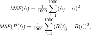
MSE( ˆα) =₁₀₀₀1 1000_∑

j=1

( ˆαj−α)2

MSE( ˆR(t)) = ₁₀₀₀1 1000_∑

j=1

( ˆR(t)_j−R(t))2,

where,αˆ andRˆ(t)are the estimates of the parameterαand the reliability function R(t), respectively. The 95% CIs of the MLEs of the parameter α and the reliability function

R(t) are computed from (29). Also, the 95% CRIs of the Bayesian and the E-Bayesian estimates of the parameter α

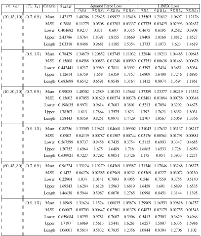
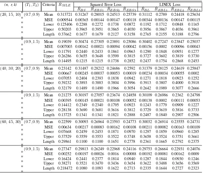
[image:4.595.352.513.74.136.2]

and the reliability function R(t) are computed from (30). All numerical results are listed in Tables (I-II). Where, in Table I,αˆEBS1,αˆEBS2andαˆEBS3stand for the E-Bayesian

estimates of α relative to SEL based on π1(a, b), π2(a, b)

andπ3(a, b), respectively,αˆEBL1,αˆEBL2andαˆEBL3denote

the E-Bayesian estimates of αrelative to LINEX based on

π1(a, b), π2(a, b) and π3(a, b), respectively. And αˆBS and

ˆ

αBLare the Bayesian estimates ofαunder SEL and LINEX loss, respectively. While in Table II, RˆEBS1, RˆEBS3 and

ˆ

REBS2 stand for the E-Bayesian estimates of R(t)relative

to SEL based onπ1(a, b),π2(a, b)andπ3(a, b), respectively,

ˆ

REBL1, RˆEBL2 and RˆEBL3 are the E-Bayesian estimates

of R(t) relative to LINEX based on π1(a, b), π2(a, b)

and π3(a, b), respectively. And RˆBS and RˆBL denote the Bayesian estimates of R(t) under SEL and LINEX loss, respectively.

VI. APPLICATION OFBURR-X MODEL

In this section, we present an illustrative example of real-life data to clarify the performance of the proposed methods in the application. These data were obtained in the Semiconductor Electronics Division of the National Institute of Standards and Technology Electronics and Electrical Engineering Laboratory and taken from [20]. This data set represents minority electron mobility for Ga1−xAlxAs semi-conductor. One data set at the mole fraction of 0.25

is considered here. This data set was used by [21], who proved that Burr-X distribution gives a good fit for this data set. The data set contains21observations as listed below. Data Set (belongs to mole fraction 0.25): 3.051,

2.779, 2.6044, 2.371, 2.214,2.045, 1.715, 1.525, 1.296,

1.154, 1.0164, 0.7948, 0.7007, 0.6292, 0.6175, 0.6449,

0.8881,1.115,1.397,1.506, and1.528.

We assume that values of data set are failure lifetime observations following Burr-X distribution. By applying UHCS on this uncensored data consideringn= 21,r= 18,

k = 15, α = 1.6526 and R(t = 1.2), we observe the following cases:

• When T1 = 1.5 and T2 = 2, we observe that k

number of failures occur afterT1, hence the experiment

is terminated at random timeT∗ =min{Xr:n, T2} = min{2.371,2}= 2.

• When T1 = 2 and T2 = 2.5, we

ob-serve that k number of failures occur before

T1, hence the experiment is terminated at

ran-dom time T∗ = min{max{Xr:n, T1}, T2} = min{max{2.371,2},2.5} = min{2.371,2.5} = 2.371.

IAENG International Journal of Applied Mathematics, 49:4, IJAM_49_4_23

(5)

• When T1 = 2.5 and T2 = 3, we

ob-serve that k number of failures occur before

T1, hence the experiment is terminated at

ran-dom time T∗ = min{max{Xr:n, T1}, T2} =

[image:5.595.94.501.148.625.2]

min{max{2.371,2.5},3}=min{2.5,3}= 2.5. With respect to the real data set, all estimates are derived based on SEL and LINEX loss functions by the same previous methods and listed in Tables (III-IV).

TABLE I: Average estimates, MSE and 95%CIs and CRIs of MLEs, Bayesian and E-Bayesian estimates forαunder LINEX and SEL functions whenα= 1.15, a= 0.8, b= 0.7, h= 1.5, c= 1.

(n, r, k) (T1, T2) Criteria αˆM LE Squared Error Loss LINEX Loss

ˆ

αBS αˆEBS1 αˆEBS2 αˆEBS3 αˆBL αˆEBL1 αˆEBL2 αˆEBL3

(20,15,10) (0.7,0.9) Mean 1.42127 1.40206 1.25625 1.09922 1.15418 1.35505 1.21812 1.0697 1.12176

MSE 0.2888 0.11275 0.0508 0.03283 0.03337 0.07775 0.03425 0.02993 0.02637

Lower 0.404682 0.9277 0.871 0.697 0.3315 0.4675 0.6195 0.2582 0.3908

Upper 2.43786 1.8764 1.8391 1.8155 1.8669 1.8408 1.8168 1.8812 1.8527

Length 2.03318 0.9488 0.9681 1.1185 1.5354 1.3733 1.1973 1.623 1.4619

(0.9,1.5) Mean 0.78429 1.34879 1.20852 1.05745 1.11032 1.32846 1.19213 1.04485 1.09645

MSE 0.15808 0.04588 0.00853 0.01248 0.00589 0.03751 0.00638 0.01463 0.00678

Lower 0.442441 1.0217 0.9989 0.7811 0.3992 0.5397 0.7434 0.3651 0.5034

Upper 1.12614 1.6759 1.658 1.6359 1.7157 1.6809 1.6408 1.7246 1.6895

Length 0.683698 0.6542 0.6591 0.8548 1.3164 1.1412 0.8974 1.3594 1.1861

(40,30,20) (0.7,0.9) Mean 0.99085 1.40502 1.2589 1.10153 1.15661 1.37389 1.23377 1.08219 1.13532

MSE 0.15602 0.07055 0.01629 0.00574 0.00378 0.05481 0.01084 0.00758 0.00348

Lower 0.198635 0.9971 0.9614 0.7603 0.3801 0.5213 0.7054 0.3292 0.4675

Upper 1.78307 1.813 1.7864 1.7575 1.823 1.792 1.7621 1.8352 1.8031

Length 1.58443 0.8159 0.8251 0.9971 1.4429 1.2707 1.0567 1.5059 1.3356

(0.9,1.5) Mean 0.88756 1.33505 1.19621 1.04668 1.09902 1.31043 1.17632 1.03137 1.08217

MSE 0.0902 0.04139 0.00787 0.01507 0.00744 0.03176 0.00561 0.01791 0.00881

Lower 0.567599 0.9737 0.9458 0.7435 0.3754 0.5115 0.6993 0.3347 0.4685

Upper 1.20752 1.6964 1.675 1.6489 1.718 1.6865 1.6533 1.728 1.6959

Length 0.639921 0.7227 0.7292 0.9054 1.3426 1.175 0.954 1.3933 1.2274

(60,45,30) (0.7,0.9) Mean 0.96224 1.33124 1.19279 1.04369 1.09587 1.31346 1.17846 1.03268 1.08375

MSE 0.1472 0.06276 0.02585 0.02969 0.0232 0.05369 0.0227 0.03072 0.0230

Lower 0.22904 1.034 1.0141 0.7893 0.4055 0.546 0.7559 0.3755 0.5140

Upper 1.69543 1.6284 1.6128 1.5963 1.6819 1.6458 1.601 1.6899 1.6535

Length 1.46638 0.5944 0.5987 0.8070 1.2765 1.0998 0.8451 1.3144 1.1395

(0.9,1.5) Mean 1.18969 1.31624 1.1524 1.00835 1.05876 1.29909 1.16553 0.99818 1.04757

MSE 0.06007 0.05703 0.00647 0.02501 0.01378 0.04873 0.02175 0.02755 0.01543

Lower 0.659684 1.0255 0.9781 0.7607 0.3906 0.5413 0.7503 0.3629 0.4966

Upper 1.7197 1.6069 1.5613 1.5441 1.6261 1.6257 1.5807 1.6335 1.5986

Length 1.06001 0.5814 0.5832 0.7835 1.2356 1.0844 0.8304 1.2706 1.102

IAENG International Journal of Applied Mathematics, 49:4, IJAM_49_4_23

(6)

[image:6.595.95.509.81.431.2]

TABLE II: Average estimates, MSE and95%CIs and CRIs of MLEs, Bayesian and E-Bayesian estimates forR(t= 1.2)

under LINEX and SEL functions whenα= 1.15,a= 0.8,b= 0.7,h= 1.5, c= 1.

(n, r, k) (T1, T2) Criteria RˆM LE Squared Error Loss LINEX Loss

ˆ

RBS RˆEBS1 RˆEBS2 RˆEBS3 RˆBL RˆEBL1 RˆEBL2 RˆEBL3

(20,15,10) (0.7,0.9) Mean 0.313721 0.31267 0.28015 0.24513 0.25739 0.31112 0.2789 0.24418 0.25634 MSE 0.009544 0.00365 0.00144 0.00147 0.00118 0.00344 0.00136 0.00147 0.00115 Lower 0.125406 0.2288 0.2272 0.1738 0.0872 0.1192 0.1712 0.0848 0.1165 Upper 0.50203 0.3965 0.3951 0.3865 0.4030 0.3956 0.3867 0.4036 0.3961 Length 0.37662 0.1677 0.1679 0.2127 0.3158 0.2765 0.2155 0.3188 0.2796

(0.9,1.5) Mean 0.19039 0.30474 0.27305 0.23891 0.25086 0.30402 0.27247 0.23847 0.25037 MSE 0.007003 0.00162 0.00021 0.00094 0.00042 0.00156 0.0002 0.00096 0.00043 Lower 0.11791 0.2440 0.2433 0.1861 0.0963 0.1290 0.1848 0.0951 0.1277 Upper 0.26286 0.3655 0.3648 0.3599 0.3815 0.3727 0.3602 0.3819 0.3730 Length 0.14495 0.1215 0.1215 0.1738 0.2852 0.2437 0.1754 0.2868 0.2453

[image:6.595.95.502.470.587.2]

TABLE III: For real data set : Average estimates, MSE and95%CIs and CRIs of MLEs, Bayesian and E-Bayesian estimates forαunder LINEX and SEL functions whenα= 1.66,a= 0.8,b= 1.4,h= 1.5, c= 2

(n, r, k) (T1, T2) Criteria αˆM LE Squared Error Loss LINEX Loss

ˆ

αBS αˆEBS1 αˆEBS2 αˆEBS3 αˆBL αˆEBL1 αˆEBL2 αˆEBL3

(21,18,15) (2,2.5) Mean 2.21753 2.45016 2.19534 1.92092 2.01697 2.26428 2.04457 1.80418 1.88877 MSE 0.87139 0.62438 0.28662 0.0681 0.12745 0.36518 0.14792 0.0208 0.05235 Lower 0.576875 1.421 1.1725 1.0514 0.4597 0.6827 0.7441 0.1725 0.3821 Upper 3.85818 3.4793 3.356 3.3393 3.3822 3.3512 3.345 3.4358 3.3954 Length 3.28131 2.0584 2.1835 2.288 2.9225 2.6685 2.6009 3.2633 3.0133

(2.5,3) Mean 2.15877 2.44508 2.19079 1.91694 2.01279 2.26161 2.04193 1.80164 1.88619 MSE 0.7657 0.61638 0.28177 0.06604 0.12449 0.362 0.14592 0.0201 0.0512 Lower 0.58324 1.422 1.1772 1.0528 0.4615 0.6844 0.7493 0.1777 0.3873 Upper 3.7343 3.4681 3.346 3.3288 3.3724 3.3412 3.3346 3.4256 3.385 Length 3.15106 2.0461 2.1688 2.276 2.9108 2.6567 2.5853 3.2478 2.9977

TABLE IV: For real data set : Average estimates, MSE and95%CIs and CRIs of MLEs, Bayesian and E-Bayesian estimates forR(t= 1.2)under LINEX and SEL functions, α= 1.66,a= 0.8,b= 1.4,h= 1.5, c= 2.

(n, r, k) (T1, T2) Criteria RˆM LE Squared Error Loss LINEX Loss

ˆ

RBS RˆEBS1 RˆEBS2 RˆEBS3 RˆBL RˆEBL1 RˆEBL2 RˆEBL3

(21,18,15) (2,2.5) Mean 0.472972 0.51653 0.46281 0.40496 0.42521 0.51237 0.45947 0.4024 0.42239 MSE 0.025538 0.01504 0.00475 0.00012 0.00098 0.01404 0.0043 0.00007 0.00081 Lower 0.168667 0.3706 0.3662 0.2829 0.1421 0.1943 0.2756 0.1353 0.1871 Upper 0.77727 0.6625 0.6585 0.6428 0.6679 0.6562 0.6433 0.6695 0.6576 Length 0.60861 0.2919 0.2923 0.3599 0.5258 0.4619 0.3677 0.5342 0.4705

(2.5,3) Mean 0.46478 0.51586 0.46221 0.40443 0.42465 0.51173 0.4589 0.4019 0.42186 MSE 0.02316 0.01488 0.00467 0.00011 0.00095 0.01389 0.00423 0.00006 0.00078 Lower 0.169633 0.3706 0.3663 0.2829 0.1421 0.1943 0.2757 0.1355 0.1872 Upper 0.75993 0.6611 0.6572 0.6415 0.6667 0.655 0.6421 0.6683 0.6565 Length 0.59030 0.2905 0.291 0.3587 0.5246 0.4607 0.3664 0.5329 0.4692

IAENG International Journal of Applied Mathematics, 49:4, IJAM_49_4_23

[image:6.595.93.504.629.752.2]

(7)

VII. CONCLUDING REMARKS

In this paper, we used the maximum likelihood method, as well as the Bayesian and the E-Bayesian approaches, for estimating the unknown parameter and the reliability function of Burr-X distribution based on UHCS. The Bayesian and E-Bayesian estimates are derived under the SEL and the LINEX loss functions. The MCMC algorithm is applied to obtain the Bayesian and the E-Bayesian estimates as they cannot be obtained analytically. Also, we constructed the CIs of MLEs and the CRIs of the Bayesian and the E-Bayesian estimates. Furthermore, an illustrative example is presented to investigate the performance of the proposed methods in the application. Based on the results obtained in Tables (I-II), we observe the following.

• The Bayesian estimator is better than MLE in terms of MSE.

• The E-Bayesian estimator is the best when compared with the Bayesian and the MLEs in the sense of having a smaller MSE.

• The MSE of all estimates decreases when the sample size nand time pointsT1, T2 increase.

• Also, the length of CIs and CRIs decreases when

n, r, T1andT2 increase.

• The E-Bayesian estimator is more efficient than the Bayesian and MLEs, as it has a smaller MSE.

• Based on the results obtained in Tables (III-IV), we observe that all the previous results are realized for the Bayesian, the E-Bayesian estimates and MLEs, that is the proposed methods behave well for a practical real data set.

• Moreover, the E-Bayesian estimator is the most efficient compared with the Bayesian estimator and MLE in the application.

• On the other hand, the length of CIs and CRIs decreases when n, r, T1 andT2 get larger.

• From Tables (I-IV), we can state that the E-Bayesian method is easy to apply and more efficient than both Bayesian and maximum likelihood methods.

• Also, a large sample sizen gives better estimates with a smaller MSE.

• Furthermore, the E-Bayesian method can be applied to any censoring scheme as performed in [11], [16] and [17] with the same efficient behavior.

ACKNOWLEDGMENT

The authors would like to thank the associate editor, the editor and the referees for their constructive comments and suggestions that improved the content and the style of this paper.

REFERENCES

[1] B. Chandrasekar, A. Childs and N. Balakrishnan, “Exact likelihood inference for the exponential distribution under generalized Type-I and Type-II hybrid censoring,”Naval Research Logistics,vol. 51, no. 7, pp. 994-1004, 2004.

[2] B. Epstein, “ Truncated life tests in the expoential case,”Annals of Mathematical Statistics,vol. 25, no. 3, pp. 555-564, 1954.

[3] N. Balakrishnan, A. Rasouli and N. Sanjari Farsipour, “Exact likelihood inference based on an unified hybrid censored sample from the expo-nential distribution,”Journal of Statistical Computation and Simulation,

vol. 78, no. 5, pp. 475-488, 2008.

[4] N. Balakrishnan, D. Kundu, “Hybrid censoring: models, inferential results and applications,” Computational Statistics & Data Analysis,

vol. 57, no. 1, pp. 166-209, 2013.

[5] W.T. Huang and K.C. Yang, “A new hybrid censoring scheme and some of its properties,” Tamsui Oxford Journal of Information and Mathematical Sciences,vol. 26, no. 4, pp. 355-367, 2010.

[6] R.A. Habibi, M. Izanlo, “An EM algorithm for estimating the param-eters of the generalized exponential distribution under unified hybrid censored data,”Journal of Statistical Research of Iran,vol. 8, no. 2, pp. 149-162, 2011.

[7] H. Panahi and A. Sayyareh, “Estimation and prediction for a unified hybrid-censored Burr Type XII distribution,” Journal of Statistical Computation and Simulation,vol. 86, no. 1, pp. 55-73, 2016. [8] W. I. Burr, “Cumulative frequency distribution,”Annals of Mathematical

Statistics,vol. 13, no. 2, pp. 215-232, 1942.

[9] A. Y. Al-Hossain, “Burr-X model estimate using Bayesian and non-Bayesian approaches,”Journal of Mathematics and Statistics,vol. 12, no. 2, pp. 77-85, 2016.

[10] A. A. Ahmad, M. E. El-Adll and T. W. AlOafi, “Estimation under Burr type X distribution based on doubly type II censored sample of dual generalized order statistics,”Journal of the Egyptian Mathematical Society,vol. 23, no. 2, pp. 391-396, 2015.

[11] A. Rabie and J. Li, “E-Bayesian estimation for Burr-X distribution based on Type-I hybrid censoring scheme,”IAENG International Jour-nal of Applied Mathematics,vol. 48, no. 3, pp. 244-250, 2018. [12] M. Han, “The structure of hierarchical prior distribution and its

applications,”Chinese Operation Research and Management Science,

vol. 6, no. 3, pp. 31-40, 1997.

[13] M. Han, “E-Bayesian estimation and hierarchical Bayesian estimation of failure rate,”Applied Mathematical Modelling, vol. 33, no. 4, pp. 1915-1922, 2009.

[14] Z. F. Jaheen and H. M. Okasha , “E-Bayesian estimation for the Burr Type XII model based on Type II censoring,”Applied Mathematical Modelling,vol. 35, no. 10, pp. 4730-4437, 2011.

[15] H. M. Okasha, “E-Bayesian estimation for the Lomax distribution on Type-II censored data,”Journal of the Egyptian Mathematical Society,

vol. 22, no. 3, pp. 489-495, 2014.

[16] A. Rabie and J. Li, “E-Bayesian estimation for the Burr-X dis-tribution based on generalized Type I hybrid censoring scheme,”

American Journal of Mathematical and Management Sciences,2019, doi:10.1080/01966324.2019.1579123.

[17] A. Rabie and J. Li, “E-Bayesian Estimation Based on Burr-X Gen-eralized Type-II Hybrid Censored Data,”Symmetry,vol. 11, no. 5, pp. 1-14, 2019.

[18] M. K. Cowles and B. P. Carlin, “Markov chain Monte Carlo diagnos-tics: a comparative review,”Journal of American Statistical Association,

vol. 91, no. 434, pp. 883-904, 1995.

[19] W. K. Hastings, “Monte Carlo sampling methods using Markov chains and their applications,”Biometrika,vol. 57, no. 1, pp. 97-109, 1970. [20] H. S. Bennett and J. J. Filliben, “A Systematic approach for

multidi-mensional, closed-form analytic modeling: minority electron mobilities inGa1−xAlxAshetero structures,”Journal of Research of the

Nation-al Institute of Standards and Technology,vol. 105, no. 3, pp. 441-452, 2000.

[21] B. Tarvirdizade and H. K. Gharehchobogh, “Inference on Pr(X > Y)

based on record values from the Burr Type X distribution,”Hacettepe Journal of Mathematics and Statistics,vol. 45, no. 1, pp. 267-278, 2016.