Guiding Optical Flow Estimation

Guiding Optical Flow Estimation

Peter J. Myerscough, Mark S. Nixon, and John N. Carter

Department of Electronics and Computer Science,

University of Southampton,

Southampton, SO17 1BJ, UK

[pjm01r|msn|jnc]@ecs.soton.ac.uk

Abstract

We show how optical flow estimates can be combined with boundary esti-mation to improve estimates of motion. The improvement is associated with blending of estimates from complementary bases of operation. The paper combines a phase-based method for optical flow with a time extended ver-sion of the phase congruency operator. By evaluation on synthetic and real image sequences, the combination of the two techniques is shown to im-prove motion estimation with particular advantages at motion boundaries, regions which have posed considerable difficulty for previous motion esti-mation techniques. The advantage is derived using the moving feature infor-mation in an extended phase congruency operator to constrain correct data in the optical flow field.

1

Introduction

Motion blur is a real problem for optical flow calculation. Most optical flow techniques use operations on groups of pixels to calculate the optical flow at a particular point. To justify this, an assumption of a single motion field, (or a smoothly varying motion field) model is used. If, however, within a group of pixels there is a motion boundary, or multiple motions violate this assumption, then the resulting field will be biased or erroneous. We show that it is possible to use motion boundary information to separate motion fields and reduce or remove blurring across such boundaries.

Knowing that both optical flow and motion boundary estimation can be computation-ally expensive, two techniques that are phase-based have been chosen as a basis for this work. The first is phase-based optical flow developed by Fleet and Jepson [4]. It provides dense flow fields and sub-pixel accuracy. In a review by Barron [2] it was shown to pro-duce good results in comparison to a number of other techniques. The second is a robust feature detector which uses phase congruency, developed by Kovesi [6]. This technique is designed for image feature detection, but has been extended here to detect features that persist over time.

1.1

Phase-based Optical Flow

Fleet and Jepson[4] propose that the flow of the phase values of an image sequence’s component frequencies is synonymous with the optical flow of the sequence. The first step of the technique is the convolution of a series of Gabor filters, N(x;y;t;ωx

i;ωy

i;ωt

(with zero DC response), with the image sequence, I(x;y;t)as in eqn. 1 to obtain filtered

images , Ri(x;y;t), as

Ri(x;y;t)=I(x;y;t)N(x;y;t;ωx

i;ωy

i;ωt

i) (1)

where

N(x;y;t;ωx;ωy;ωt) = G(x;y;t)(e

i(ωxx+ωyy+ωtt)

e b2=2

) (2)

G(x;y;t) =

1 2πσ

3=2

e

((x x0)

2

+(y y0)

2

+(t t0)

2

)

2σ2 ₍₃₎

b =

2β+1

2β 1 (4)

andβ is a measure of the bandwidth the filter has oneσ from its centre. There are 22 sets of constantsωxi;ωy

i;andωt

i which orientate the filtering at six 30

Æ

intervals with

ωti =0, ten 36 Æ

intervals withωti =1= p

3, and six 60Æ

intervals withωti = p

3. The Gaussian envelopes are centred at(x0;y0;t0). This produces a set of complex responses

for frequencies at various orientations in the sequence containing phase and amplitude information. The differentials of these responses about each axis [∇Rx(x;y;t),∇Ry(x;y;t)

, ∇Rt(x;y;t)] are then calculated using a 5-point complex central differencing kernel.

These are then combined to produce an estimate of the phase gradient about each axes, ∇φx(x;y;t),∇φy(x;y;t)and∇φt(x;y;t), using the identity in equation 5.

δlog(R(x;y;t))

δx =

R

(x;y;t)∇Rx(x;y;t) jR(x;y;t)j

2 =

∇ρx(x;y;t)

ρ(x;y;t)

+i:∇φx(x;y;t) (5)

where R

(x;y;t)is the complex conjugate of the response, R(x;y;t). This in turn enables

the component velocity, ˜V(x;y;t), to be calculated as in equation 6.

˜

V(x;y;t) =

(∇φx(x;y;t)∇φt(x;y;t)

∇φx(x;y;t)

2

+∇φy(x;y;t)

2;

(∇φy(x;y;t)∇φt(x;y;t)

∇φx(x;y;t)

2

+∇φy(x;y;t)

2

(6)

The results are also thresholded dependent upon conditions that eliminate phase sin-gularities [5] and points where the response to the Gabor filter is too small and possibly dominated by noise. A final step of applying a least squares operation on a local neigh-bourhood of component velocities produces full 2D velocity estimates.

1.2

Phase Congruency

Phase congruency is a robust feature detector. It detects not only step and line responses, but also a broader set of features [1]. Its attributes include a high degree of invariance to lighting variation within images. This paper extends the phase congruency technique to work with image sequences. The technique’s first step is to convolve the image with a set of log-Gabor filters at ’l’ different orientations and ’m’ different scales. Log-Gabor filters are chosen because they have zero DC response, and in cosine and sine based pairs they have a quasi-quadrature relationship. At each orientation a measure of the spread of energy amongst the different scales, wn(x;y), is calculated.

wn(x;y)=

An(x;y)

m(Amax(x;y)+ε)

where An(x;y)is the amplitude of the response to the quadrature pair of filters at scale

n and Amax(x;y)is the maximum amplitude response for the set of log-Gabor filters at

all orientations. εis a small constant avoiding division by zero which ensures that if the amplitude at a pixel becomes too small it is masked out. This is then mapped through a sigmoid function to produce Wn(x;y)

Wn(x;y)=

1 1+e

(c wn(x;y))g

(8)

where c and g control the mapping of wn(x;y)to Wn(x;y). Also an estimate of the

level of noise at the different scales, T , is calculated[6]. Then phase congruency, PC, at each orientation, PCl, is calculated from the vector sum of the log-Gabor filter responses, Ri.

PCl(x;y) =

m

∑

n

An(x;y)

cos(∆φn(x;y) ) jsin(∆φn(x;y) )j

T

Wn(x;y)

m

∑

n

An(x;y)+ε

(9)

∆φn(x;y) = φn(x;y) φ¯(x;y) (10)

whereφn(x;y)is the phase at point(x;y)for scale n and ¯φ(x;y)is the mean phase

across all scales at that point. The use ofbcdepict that if the quantity between is negative

it is set to zero. The vector sum is thresholded by the noise level estimate, T , and scaled by the measure of the spread of the energy mapped through a sigmoid function, Wn(x;y).

This is then divided by the total energy at the chosen orientation to produce a measure of phase congruency, PCl, for that orientation. Repeating and summing of the results for

the ’l’ orientations gives the phase congruency measure for the image, PC(x;y).

PC(x;y)=

l

∑

2

Method

2.1

Temporal Phase Congruency

We now extend phase congruency to use inter-frame data to enable estimation of moving features with resilience to noise. The original technique looked for features in a two-dimensional image and used filters that were built from a one-two-dimensional signal, the log Gabor function. This was convolved with an orthogonal spreading function, in this instance the Gaussian function. An additional spreading function (orthogonal to the two original functions) can be used to create a three-dimensional (2D+T) filter to enable the detection of moving features. The measures for the estimation of noise, and energy spread are also extensible to image sequences. The original log Gabor function is

lg(ω;ωi)= (

1

p

2πσe

log(ω=ω

i)

2 log(σ=ωi) ω 6=0

0 ω=0

whereω is frequency, andωi is the tuning frequency of the filter. σ controls the

spread of the filter.

This filter is convolved in the time domain ( multiplied in the frequency domain) as in equation 13 for 2D filtering and as in equation 14 for 2D+T filtering. The filters are based upon a polar co-ordinate method for making log-Gabor filters, with the two orthogonal Gaussian spreading functions operating in the angular axes, and the log-Gabor filter about the radius or magnitude of frequency axis.

lg2Di(ω;θ;ωi;θi) =

1

p

2πσe

(θ θ

i)

2 2σ2 _lg

(ω;ωi) (13)

lg2D+Ti(ω;θ;ψ;ωi;θi;ψi) =

1 2πσe

(θ θ

i)

2 2σ2 e

(ψ ψ

i)

2

2σ2 lg(ω;ωi)

(14)

whereωrepresents the spatial or spatio-temporal frequency,θ represents the spatial angle of that frequency andψrepresents the temporal angle in frequency space.θiandψi

are the angles the filters are focused upon, and againσcontrols the spread of the filters. This extension to phase congruency has two main advantages. The first advantage is found in the orientation at which phase congruency is detected at a particular pixel. This describes not only its spatial, but also its temporal orientation. This is the same as describing its velocity. Therefore all features extracted with the extended method have this additional attribute already defined.

Secondly the technique should be more robust to noise. This gain in robustness is justified by examining the feature that the filters respond to. In the one-dimensional case the filters are responding at a point. In the two-dimensional case the filters are responding at a point, which if part of a feature will likely be surrounded by valid feature points in a line on either side, that by themselves would cause a minor response to the filter due to the Gaussian spreading function. This improves the signal-to-noise ratio when processing an image. Therefore when considering a point in 2D+T space, the supporting responses of a point’s neighbours in both spatial and temporal directions should increase the robustness.

2.2

Guiding Optical Flow Estimation

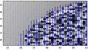
Optical flow operators suffer from motion blurring since at a boundary the estimates for motion can become mixed between one moving object and another. This is because opti-cal flow operators typiopti-cally use neighbourhood operations to compute velocity estimates or in filtering stages. Both of these occur in Fleet’s technique. An example of motion blurring can be seen in figure 1 where it is possible to see that the estimates for motion in the image blur across the boundary of the circle onto the stationary (smoothly varying) background. With a moving feature detector, it should be possible to define where the motion boundary is. With this information it is then possible to erode the motion field back towards the motion boundary, reducing errors in the motion field produced.

The erosion process uses the current velocity estimates, v, the original velocity esti-mates, vorig, and the phase congruency measures, pc to produce the new estimate, v0

Figure 1: This figure shows part of a frame from a sequence of a moving circle with the motion vectors superimposed on each pixel

v0 (x;y)=

8 <

:

incorrect [jv(x;y) v(a;b)j>λ1^vorig(x;y)>vorig(a;b)]

a;b2R ^ [pc(c;d)<λ2]

c;d2R

correct in all other cases

(15)

Co-ordinates(x;y)are those of the current point being considered,(a;b)are the nearest

points to(x;y)in direction of the motion at that point. Points(c;d)are the points ’north’,

’south’, ’east’ and ’west’ of the current. λ1 controls variation in the velocities. Previ-ous values that have been deemed incorrect are always ’different’ from another velocity estimate.λ2controls how significant a feature needs to be before it stops the erosion pro-cess. In our studies, phase congruency values greater than 0.33 are significant. Testing the original velocities means that the erosion having started from a motion boundary only creeps in one direction, that of the faster moving region. This is prescribed because faster moving regions should have a larger motion blur. Future work needs to examine more complex motion boundaries to ensure this is a valid and useful assumption.

3

Results

3.1

Temporal Phase Congruency

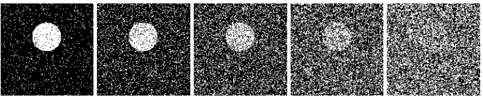
The new temporal phase congruency has been tested against the original phase congru-ency technique on a synthetic sequence of moving circles. The first test has been using a simple visual comparison. Both techniques extracted the edges of this simple image sequence very well. To gain a deeper insight, salt and pepper noise was added to the sequence in increments of 10%. At 50% salt and pepper noise, half of the pixels are set arbitrarily to black or white. Examples of the middle frame of the sequence with different noise levels are shown in figure 2.

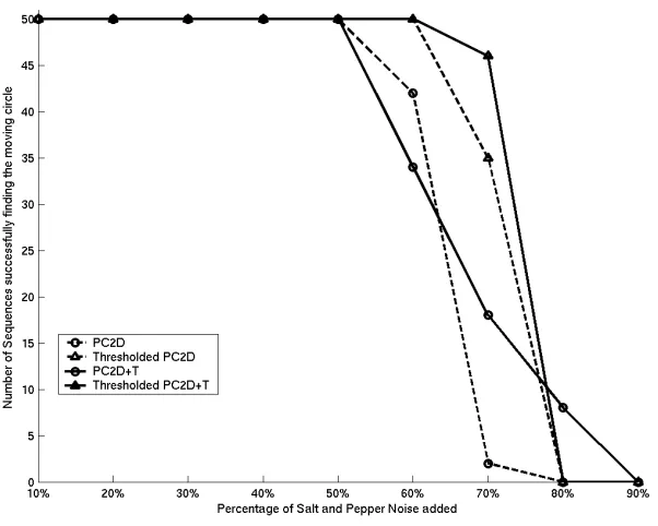
The resulting ’feature’ maps are then passed through a velocity Hough transform[7], which is a robust moving circle detector. In the results shown in figure 3 only the high-est point in the accumulator for that sequence was a correct identification of the circle’s velocity, and position. Anything different was considered a fail, a harsh judgement, but illustration enough of the performance possible here.

Figure 2: An example frame with 10%, 30%, 50%, 70% and 90% salt and pepper noise.

result obtained is more for the new technique and all except one exceed that of the original version. The lower results at 60% noise for the temporal phase congruency method when compared to the image based method could be attributed to too small a test set, but merits further investigation.

3.2

Guided Optical Flow

To test the new guided optical flow two sequences were used. The first was of a generated disc with a fixed random texture moving on a linearly varying background or ’slope’. The second was from the Southampton Gait Database [8], and involved a person walking on a green background. This sequence was processed three times using the separate red, green and blue channels, with the final flow fields being assimilated to produce a more dense flow field, than if either a grayscale sequence or a single colour channel was used. The densities of the flow fields even after combining the three channels were still too low. This is because Fleet’s technique can only detect motion up to 2 pixels per frame without sub-sampling the images. Accordingly, another optical flow technique by Bulthoff [3] was used to buttress the density of the optical flow estimates. Differences in the density of results can be seen in figure 4.

It was assumed that within the circumference of the circle and the person were the only pixels that should contain any movement. In this way the results for this test were in four categories:

- Correct results, non-zero velocity estimates only within the ’shapes’.

- False zero velocity estimates where velocity estimates should be higher than zero

- False non-zero velocity estimates where background estimates should be shown

Figure 3: Graph comparing the phase congruency and temporal phase congruency.

(a) Original Image (b) Fleet(phase) (c) Bulthoff(correlation)

Iteration Total Correct False Zero False Positive Unclassified

No. No. Percent No. Percent No. Percent No. Percent

0 224660 94.80% 186 0.08% 12146 5.13% 0 0.00%

1 224659 94.80% 186 0.08% 9700 4.09% 2447 1.03%

2 224583 94.76% 186 0.08% 8088 3.41% 4135 1.74%

3 224409 94.69% 186 0.08% 7440 3.14% 4957 2.09%

4 224274 94.63% 186 0.08% 7260 3.06% 5272 2.22%

5 224168 94.59% 186 0.08% 7213 3.04% 5425 2.29%

6 224132 94.57% 186 0.08% 7180 3.03% 5494 2.32%

7 224114 94.57% 186 0.08% 7157 3.02% 5535 2.34%

8 224100 94.56% 186 0.08% 7134 3.01% 5572 2.35%

9 224087 94.55% 186 0.08% 7111 3.00% 5608 2.37%

10 224081 94.55% 186 0.08% 7088 2.99% 5637 2.38%

11 224080 94.55% 186 0.08% 7076 2.99% 5650 2.38%

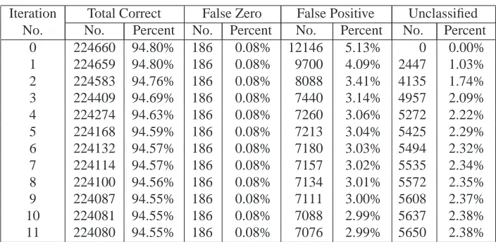
Table 1: Results from a sequence of images with a textured circle moving on a smoothly varying background

Iteration Total Correct False Zero False Positive Unclassified

No. No. Percent No. Percent No. Percent No. Percent

0 9139 55.78% 3261 19.90% 2283 13.93% 1701 10.38%

1 8945 54.60% 3223 19.67% 1976 12.06% 2240 13.67%

2 8816 53.81% 3195 19.50% 1784 10.89% 2589 15.80%

3 8737 53.33% 3164 19.31% 1668 10.18% 2815 17.18%

4 8670 52.92% 3138 19.15% 1585 9.67% 2991 18.26%

5 8614 52.58% 3116 19.02% 1530 9.34% 3124 19.07%

6 8560 52.25% 3103 18.94% 1479 9.03% 3242 19.79%

7 8516 51.98% 3095 18.89% 1439 8.78% 3334 20.35%

8 8481 51.76% 3082 18.81% 1404 8.57% 3417 20.86%

9 8454 51.60% 3067 18.72% 1380 8.42% 3483 21.26%

10 8431 51.46% 3055 18.65% 1364 8.33% 3534 21.57%

11 8416 51.37% 3041 18.56% 1349 8.23% 3578 21.84%

In both table 1 and table 2 the errors produced by the initial optical flow techniques are reclassified as ’unclassified’. This removes false confidences in the original data. The number of reclassifications is higher in the first few iterations, but the process stabilises and areas of blur are reduced to phase congruency boundaries.

(a) Flow Superimposed (b) After Erosion

Figure 5: Segments from the moving circle sequence with flow fields superimposed

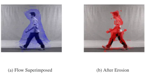
(a) Flow Superimposed (b) After Erosion

Figure 6: Flow fields for the central frame of the walking person sequence.

4

Conclusions

Results from a moving feature extraction technique can be used to guide selection of correct optical flow estimates thus improving the quality of motion extraction. The tests shown are currently single objects moving on a stationary background and reclassification of velocity vectors removes erroneous vectors. Future work should include multiple ob-jects passing behind and in front of each other, as well as more complex motion junctions. In developing this combination of motion detection, an enhanced form of the phase congruency operator has been developed. This shows improvements over the original operator in noisy conditions, although further work to remove some anomalies may be necessary. It also provides velocity information for the moving features detected. Inclu-sion of this motion information in the combined algorithm should also be a future work.

Preliminary studies on real image data were hampered by the sparsity of flow esti-mates, in part due to the large motions in the test sequences. Currently fast motion causes problems in obtaining sufficiently dense optical flow fields. This may be over come by pyramid decomposition of the image sequence, along with a method for recombining multiple scales of velocity estimates. This and other aspects merit future investigation.

Acknowledgements

This research has be funded by the EPSRC, with additional support from European Re-search Office of the US Army, Contract No.N68171-01-C-9002.

References

[1] Y. K. Aw, R. Owens, and J. Ross. A catalog of 1-d features in natural images. CVGIP:

Graphical Models and Image Processing, 56(2):173–181, March 1994.

[2] J.L. Barron, D.J. Fleet, and S.S. Beauchemin. Performance of optical flow techniques.

International Journal of Computer Vision, 12(1):43–77, 1994.

[3] H. Bulthoff, J. Little, and T. Poggio. A parallel algorithm for real-time computation of optical-flow. Nature, 337(6207):549–553, February 1989.

[4] D.J. Fleet and A.D. Jepson. Computation of component image velocity from local phase information. International Journal of Computer Vision, 5(1):77–104, 1990.

[5] D.J. Fleet and A.D. Jepson. Stability of phase information. IEEE Trans. PAMI, 15(12):1253–1268, December 1993.

[6] P Kovesi. Image features from phase congruency. Videre : Journal of Computer

Vision Research, 1(3):1–27, 1999.

[7] J. M. Nash, J. N. Carter, and M. S. Nixon. Dynamic feature extraction via the velocity hough transform. Pattern Recognition Letters, 18:1035–1047, 1997.