Alternative Pricing Methods for Shout Call Options

Alternative Pricing Methods for Shout Call

Options

Joanna Goard

Abstract—Shout call options are exotic options that give the investor the ability to ‘shout’ during the life of the option, thus locking in a profit and resetting the strike price to the prevailing spot price. We look at two approaches to value such options. The first approach makes use of canonical variables of the clas-sical heat equation and results in a series solution. In the second approach an integral formulation is used, which can be more amenable to pricing when there is more than one ‘shout’ allowed.

Keywords: shout options, strike reset options

1

Introduction

In general, a shout option allows the holder of the option to ‘shout’ at one or more times during the life of the option and so adjust certain aspects of the option such as the strike price or time to maturity. In their original form however (and possibly still the more well-known form, see e.g.[2]), shout contracts permit the holder to ‘shout’, in which case the strike price is reset to the then prevailing spot price and a payment at expiry to the holder is locked-in of max(St−X,0), whereSt is the current asset price

andXthe strike price. This is further to the usual payoff from the option using the new strike price. Some shout options offer the holder to shout more than once, and the general rule is that if annshout option is exercised early at time t, the holder receives max(St−X,0) for a call

(at expiry) along with a new at-the-money (n−1) shout option.

The shouting right of the holder necessarily gives rise mathematically to a free boundary problem. Daiet al[1] provide an exact representation for the price of a shout floor (which is a special case of the strike reset put (see Section 2) in which the initial strike price is set at zero), and derived a (double) integral representation for a shout-ing premium for a reset put option. However much of the work done to date is numerical. For example, finite dif-ference methods have successfully been applied to shouts by Windcliffet al([5]). In this paper we look at two ap-proaches to formally derive valuations for shout options and their optimal shout boundaries (OSB). In the first approach the governing PDE is reduced to the classical

∗_{School of Mathematics and Applied Statistics,}

Univer-sity of Wollongong, Wollongong, NSW 2522, AUSTRALIA. [email protected]

heat equation and then we make use of the result that for any linear partial differential equation (PDE) with a Lie point symmetry, separation of variables is possible in terms of canonical symmetry coordinates (see [3]). This approach leads to a series solution for the option value. In the second approach we use an integral equation formu-lation. Both approaches have their advantages. While the first method avoids the need to integrate and finds the coefficients for the option value and OSB simultane-ously, the second approach involves the decoupling of the option valuation problem from finding the free bound-ary and would be able to handle multiple free boundaries corresponding to multiple shouts. Both methods result in the same series form for the OSB.

2

Approach 1: Series Solution for Option

Value

To price shout call options we begin by focussing on the mathematical model for the related strike reset put op-tion. A strike reset put option allows the holder of the put option to ‘shout’ during the life of the option, upon which the strike of the option is reset to the stock price at the time of the shout. Hence, if the holder does not shout during the life of the option, the payoff at expiry time T from the option is max(X −ST,0), where X is

the original exercise or strike price; whereas if a shout is made at timet, then the payoff at expiry timeT is given by max(St−ST,0). Hence the holder will only shout if St > X in order to increase the payoff value. We show

in Section 2.3 that the price of a shout call option can be derived from the price of a strike reset put option so we begin by pricing the strike reset put option.

We assume that the stock priceS(=St) follows the usual

risk-neutral lognormal process i.e

dS/S= (r−q)dt+σdZ (1)

where r, q and σ are the constant risk-free rate, divi-dend yield and volatility respectively andZ is a Wiener process under a risk-neutral measure. Upon expiry time T, the holder of the strike reset put option receives max(X−ST,0) so that the holder will shout at timet < T

only ifSt> X. Upon shouting, the option becomes an

shouting boundary,Sf(t) becomes P(S, t) =Pe(S, t;S),

wherePe(S, t;X) is the Black-Scholes formula for the

Eu-ropean put option with strikeX. In the continuation re-gion, 0≤S ≤Sf(t) the value P(S, t) of the strike reset

put option can be shown to satisfy the Black-Scholes (BS) equation

∂P ∂t +

σ2S2 2

∂2P

∂2S + (r−q)S ∂P

∂S −rP = 0 (2)

whereq is the constant, continuous dividend yield. The option price must necessarily satisfy the smooth-pasting conditions so that across the optimal shouting boundary, the value of the option and its derivative are continuous. Equation (2) then needs to be solved subject to

P(S, T) = max(X−S,0), (3a)

P(0, t) =Xe−r(T−t) (3b) and atSf(t)> X

P(Sf(t), t) =Sf(t)[e−r(T−t)N(−d2)−e−q(T−t)N(−d1)]

(3c)

PS(Sf(t), t) =e−r(T−t)N(−d2)−e−q(T−t)N(−d1) (3d)

whereT is the expiry date, N(·) is the cumulative dis-tribution function for the standard normal disdis-tribution,

d₁= (r−q+σ

2 2)

√

(T−t)

σ andd2=d1−σ

√

T−t.

In the following subsection, an exact formal solution will be given for the strike reset put option based on solving (2) subject to (3a)-(3d). The following result will be used, which was proven by Daiet al[1].

Result 2.1The optimal shouting boundary for the strike reset put option takes on the value X at expiry i.e Sf(T) =X.

2.1

Solution for the Strike Reset Put Option

Consider the value V(S, t) of a strike reset put option P(S, t) plus a forward contract f(S, t) = Se−q(T−t)− Xe−r(T−t).Because an investor will shout only ifSf(t)> X,it is worthwhile to split the continuation domain into the 2 regions 0≤S < X andX ≤S ≤Sf(t). Note that

using Result 2.1, the regionX ≤S≤Sf(t) reduces to a

single point at t=T. In the continuation region of the reset put option,V(S, t) satisfies Equation (2) which in

X≤S≤Sf(t) needs to be solved subject to

V(Sf(t), t) =Sf(t)[e−r(T−t)N(−d2) +e−q(T−t)N(d1)]

−Xe−r(T−t) (4a) VS(Sf(t), t) =e−r(T−t)N(−d2) +e−q(T−t)N(d1) (4b)

and in 0≤S < X, subject toV(S, T) = 0.

We also impose the smooth pasting conditions i.e conti-nuity of the value of the option and its derivative across the strike price i.e

lim

S→X−V = limS→X+V and S→limX−VS = limS→X+VS.

We make the following substitutions, the first two of which are the standard substitutions that reduce the BS equation to the classical heat equation:

(a) S=Xex, t=T−2τ

σ2, V =e

−q(T−t)_{Xν(x, τ), (5)}

and letG(τ) = ln

Sf(t)

X

whereG(0) = 0.

(b) u(x, τ) =eAx+Bτν(x, τ) (6) whereA = k−₂1, B = (k+1)₄ 2, resulting in the governing equationut=uxx.

(c) y=√x

τ, τ = τ (7)

which are canonical coordinates ofut=uxx.

The problem then becomes

τ uτ =uyy+y

2uy (8)

to be solved subject to u(y,0) = 0 for y < 0 and for 0≤y≤Ψ(τ),where Ψ(τ) = G√(τ_τ)

u(Ψ(τ), τ) =−eA√τΨ(τ)+Bτe−kτ +e(A+1)√τΨ(τ)+Bτ

N(d₁) +e−kτN(−d₂)

(9a)

uy(Ψ(τ), τ) =−A√τ eA

√_τ

Ψ(τ)+Bτ_e−kτ

+√τ(A+1)e(A+1)√τΨ(τ)+Bτ[N(d₁)+e−kτN(−d₂)] (9b)

lim

y→0−u= limy→0+u and (9c)

lim

y→0−uy = limy→0+uy. (9d)

Equation (8) admits separable solutions of the form

u(y, τ) =e−4y2 ∞

i=1

τ2i

CiM

1 +i

2 , 1 2,

y2

4

+DiU

1 +i

2 , 1 2,

y2

4

,

(10)

whereM andUare the Kummer-M and Kummer-U func-tions respectively. The separation constant used in (10) is λi = ₂i where i is a positive integer, as power series

consideration of the initial condition implies solutions of the form

u(y, τ) =e−4y2

∞

i=1

τ2i_FiU

1 +i 2 ,

1 2,

y2 4

(11)

for constantsFi to be determined.

Determining the Solution Coefficients

In order to satisfy the limit conditions at y = 0 we re-quire

Fi =Γ(1 + i

2)

√

π Ci+Di and (12a)

Fi =−Di (12b)

so that we setCi= −2

√_π

Γ(1+i

2)Di.

Note that for continuity at x= 0 of the second deriva-tives, we require

√

π

Γ(1 +₂i)iFi=iCi+

√

π Γ(1 +₂i)iDi

but this follows automatically from (12a). Hence deriva-tives of all orders are continuous atx= 0.

We let Ψ(τ) = ∞_i=0siτi/2. This is motivated by the

classic work of Tao (see e.g. [4]) on Stefan problems in general. Now apply (9a) and (9b) to determine the coef-ficientssi andDi, using the following steps:

(i) Using (10) expand both sides of Equation (9a) in a power series ofτi/2. We call this Expansion A.

(ii) Similarly expand both sides of Equation (9b) in a power series ofτi/2 and call this Expansion B.

Both expansions have no constant terms.

(iii) By equating coefficients of τ1/2 from both sides of Expansion A and similarly from both sides of Expansion B, yields 2 equations to solve for the unknownsD₁ and s₀. The solution to this system (to 4 decimal places) is s₀= 1.0304 andD₁=−0.3678.

Then, equating coefficients of powers of τ from Expan-sions A and B yields 2 equations to solve forD₂ ands₁. In general we can then continue equating coefficients of τi2 from Expansions A and B to get as many constantsDi

andsi−1as necessary. These coefficients will be in terms

of k=2(r_σ−2q)

. Then constants Fi can be determined

from (12b).

Undoing the change of variables (7), (6), (5) givesV(S, t). Then subtracting the value of the forward contract gives the solution forP(S, t). We thus have

Theorem 2.1:The following series formally satisfies the free boundary problem (2)-(3) for the strike reset put option in the continuation region 0≤S≤Sf(t):

P(S, t) =g(S, t)∞

i=1

σ2

2(T−t)

i/2

Di

U

1 +i

2 , 1 2,

(ln(S/X))2

2σ2₍T−t)

+ −2

√_π

Γ(1 +i

2)

M

1 +i

2 , 1 2,

(ln(S/X))2

2σ2₍T−t)

(13a)

−Se−q(T−t)_+Xe−r(T−t) _forX≤S≤S

f(t)

=−g(S, t)∞

i=1

σ2

2 (T−t)

i/2

DiU

1 +i

2 , 1 2,

(ln(S/X))2

2σ2₍T−t)

−Se−q(T−t)+Xe−r(T−t) for 0≤S < X (13b)

where

g(S, t) =e−q(T−t)X _S

X 1−k

2

e−(k+1)2σ82(T−t)e−

(ln(_XS))2 2σ2(T−t)_,

(14) k= 2(r_σ−2q), and the optimal shouting boundary is given

by

Sf(t) =Xexp ⎛ ⎝∞

i=0

si

σ2 2 (T−t)

(i+1) 2

⎞

⎠. (15)

The coefficients si and Di are determined from the

boundary conditions at Sf(t) as described above. The

first seven coefficients s₀ −s₆ for the optimal bound-ary and the first seven coefficients for the option value D₁−D₇ are listed in the Appendix.

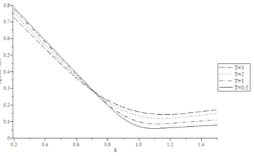
Plots showing a comparison of option values with differ-ent times to expiry using (13a, 13b) withσ= 0.2, X = 1, r= 0.03, q= 0.02 are shown in Figure 1.

Figure 1: Comparison of strike reset put prices with dif-ferent times to expiry. Parameters used wereX= 1, r= 0.03, σ= 0.2 andq= 0.02.

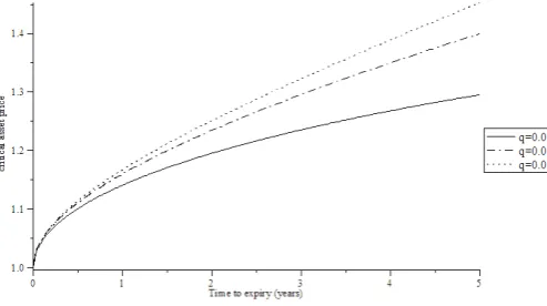
at-the-money put option at the stock price corresponding to the optimal shout boundary. A comparison of the optimal shout boundaries for differentqvalues and with X= 1 and r= 0.03, σ= 0.2 is given in Figure 2.

Figure 2: Optimal shout boundaries with parameters X= 1, r= 0.03 andσ= 0.2.

From this it can be seen that the larger the dividend yield, then the smaller the optimal shout boundary. This is to be expected as dividend yields have the effect of lowering the growth rate in the stock price. Notably also, when r < qthe optimal shout boundary has a lower slope and a greater curvature.

2.2

Examples and Comparisons

We compared results from the series truncated at seven terms, with accurate solutions for a 5 year reset put op-tion, obtained by using 50000 time steps in the Bino-mial Model, as given by Dai [1] with parameter values T−t = 5, S = 100, r = 0.06 and 0.03, q = 0.03 and 0.06, σ= 0.2 and 0.3.It was found that better accuracy was achieved with fewer terms in our formal series solu-tions when σ is larger and when r < q. However in all cases, at last 4 significant figure accuracy was achieved using seven terms.

In order to understand how many terms the series gener-ally requires in order to attain good accuracy, we tried a number of examples withT−t= 0.5,1,2,3, q= 0.06,and 0.02, r = 0.03, X = 1 and found the number of terms snneeded in Equation (15) and the number of termsDn

needed in Equations (13a) or (13b) to achieve 4 decimal place accuracy inSf(t) andP(S, t) respectively. In each

case the ‘exact’ solution was taken as the value where the

relativedifferences between successive values usingnand n+ 1 terms was less than 10−4. In every case, the prac-tical criterion for accuracy was satisfied with the number of termssn required ranging from 3 to 5 and the number

of terms Dn ranging from 2 to 5. In general, the larger

the time to expiry, the more terms were needed and when

r > qthen moresi andDiterms were sometimes needed

for the same accuracy in Sf and P. Hence for all cases

considered, the new series solutions provided fast and ac-curate answers for times to expiry up to three years.

We now use the results from this section to value shout call options.

2.3

Solution for the Shout Call Option

Theorem 2.2:

An exact formal solution for the shout call optionV(S, t) in the continuation region 0≤S ≤Sf(t) is

V(S, t) =g(S, t)∞

i=1

σ2

2 (T−t)

i/2

DiU

1 +i

2 , 1 2,

ln(S/X)2

2σ2₍T−t)

+ −2

√_πD i

Γ(1 +i

2)

M

1 +i

2 , 1 2,

ln(S/X)2

2σ2₍T−t)

(16a) forX≤S≤Sf(t)

=−g(S, t)∞

i=1

σ2

2(T−t)

i/2

D_iU

1 +i

2 , 1 2,

ln(S/X)2

2σ2₍T−t)

for 0≤S < X (16b)

where g(S, t) is given in (14), k = 2(r_σ−2q) and the

op-timal shout boundary is given by (15). The constant coefficientsDi and si are again determined as described

in Section 2.1.

Note that in the regionSf(t)> X, the value of the shout

call option is simplyCe(S, t;S) + (S−X)e−r(T−t)where Ce(S, t;X) is the Black-Scholes value of a European call

with strike priceX.

Proof: The holder of a shout call option can ‘shout’ if St> X, which resets the strike price toStand locks in a

payment they will receive at expiry of St−X. Thus,

the payoff from the shout call option is Csh(S, T) =

max(ST −X, St−X,0). As max(ST −X, St−X,0) =

max(St−ST,0) + (ST −X), then the shout call option

can be replicated using a strike reset put option and a long position in a forward contract with the same strike. Hence the value of the shout call option is simplyV(S, t) from Section 2.1 - i.e. the sum of the value of the strike reset put option and a forward contract ie.

Csh(S, t) =V(S, t) =P(S, t) +Se−q(T−t)−Xe−r(T−t)

whereP(S, t) is given in (13a, 13b). The optimal shout boundary is then the same as for the strike reset put option which is given in (15).##

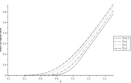
Figure 3: Comparison of shout call option prices with different times to expiry. Parameters used were X = 1, r= 0.03, q= 0.02, σ= 0.2.

3

Approach 2: An Integral Equation

For-mulation

With ˜τ =T−t,the BS equation can be written as

LV =

∂ ∂τ˜ −

σ2S2 2

∂2

∂S2 −(r−q)S ∂ ∂S +r

V = 0,(17)

where we have defined the operatorLfor later use.

For American-style options with early exercise features, it follows from an application of Green’s theorem that if such an option obeys equation (17) where it is optimal to hold the option, while that from immediate exercise is P(S,τ˜), then we can write the value of the option as the sum of the value of the corresponding European option V(e)(S,τ˜) together with another term representing the premium from early exercise,

V(S,τ˜) =V(e)(S,τ˜) +

τ_˜

0

_∞

0 F

(Z, ζ)G(S, Z,τ˜−ζ)dZdζ. (18)

whereGis the Green’s function,

G(S, Z,τ˜) = e −rτ˜

Zσ√2πτ˜exp

−[ln(S/Z) +r2τ˜]2

2σ2τ˜

(19)

and we have introduced the shorthandr₂=r−q−σ2/2. In this equation, F(S,τ˜) is equal to 0 where it is op-timal to hold the option while where exercise is opop-timal

F(S,τ˜) is the result of substituting the early exercise pay-offP(S,τ˜) into BS partial differential equation,

F(S,˜τ) =LP, (20)

where the operatorLwas defined in (17). Similarly, shout options satisfy LV = F(S,τ˜), where F = 0 when it is not optimal to shout and otherwiseF =LP where P is the payoff from shouting. Hence for shout options, we can use the formulae (18,20) recursively. We shall use the notation V(n)(S,τ˜) for the value of a shout option with n shouting opportunities and X(n) for the strike price of an n shout option. If held until expiry, an n shout call will pay max(S−X(n),0) while a put will pay max(X(n)−S,0). At the first shout, which will occur at the free boundary S_f(n)(˜τ), we exchange this n shout option for a lock-in payment at expiry of the difference between the current stock price S and the strike price X(n) together with a new at-the-money (n−1) shout optionV(n−1)(S,τ˜)|_X(n−1)₌S. At-the-money in this

con-text means that the strike priceX(n−1)of this new (n−1) shout option is set equal to the stock priceS at the time of exercise. It follows that the payoff from exercise for an nshout call is

P(n)_{(S,τ˜) = (S−X}(n)_)e−rτ˜_+V(n−1)_(S,τ˜)|

X(n−1)_=S(21)

[while for annshout put it is

P(n)(S,τ˜) = (X(n)−S)e−rτ˜+V(n−1)(S,τ˜)|_X(n−1)_=S]

An option with zero shouts remaining is just a vanilla European, V(0)(S,˜τ) = V(e)(S,τ˜). If we exercise a one shout option, we will receive at expiry the difference be-tween the stock price and the initial strike price and we receive immediately a zero shout option which is simply an at-the-money European option. So the payoff from shouting for a one shout call, withr₁=r₂+σ2, is

P(1)(S,˜τ) = (S−X(1))e−rτ˜+V(0)(S,˜τ)|X(0)₌S,

= (S−X(1))e−rτ˜ (22)

+ S 2

e−qτ˜erfc

− r1˜τ

σ√2˜τ

−e−rτ˜erfc

− r2τ˜

σ√2˜τ

,

Using (20), the forcing term in the formula (18) for a one shout call is

F(1)_{(S,τ˜) (23)}

=−S 2e

−rτ˜_(r−q)erfc r2τ˜

σ√2˜τ

−√σ

2πτ˜exp

−r22τ˜

2σ2

the value of a one shout call,

V(1)(S,˜τ) =V(e)(S,τ˜) +

τ_˜

0

_∞

S_f(1)(ζ)

−rZ 2 e

−rζ ₊qZ

2 e

−rζ_erfc r2ζ

σ√2ζ

+Zσe −rζ

2√2πζ exp

−r22ζ

2σ2

G(S, Z,τ˜−ζ)dZdζ

=Se−

q˜τ

2 erfc

−ln(S/X(1)) +r1τ˜

σ√2˜τ

−Xe−rτ˜

2 erfc

−ln(S/X(1)) +r2τ˜

σ√2˜τ

+

τ_˜

0

−(r−q) 2σ√2π√τ˜−ζe

−r˜τ_erfc

r₂√ζ σ√2

+ e−

rτ˜

4π√ζ√τ˜−ζexp

−r22ζ

2σ2

×σS

π(˜τ−ζ)

√

2 e

(r−q)(˜τ−ζ)

×erfc

ln(Sf(ζ))−ln(S)−r1(˜τ−ζ)

σ2(˜τ−ζ)

dζ. (24)

3.1

Integral Equations For One Shout

Op-tions

To obtain integral equations for the location of the free boundary S = S_f(1)(˜τ) for a one shout option we sub-stitute the expressions for the one shout call (24) into the conditions at the free boundary. To simplify the analysis, we will writeS_f(1)(˜τ) =X(1)exp

x(1)_f (˜τ)

, not-ing as in Section 2 that the free boundary starts from S_f(1)(0) = X(1) or equivalently x(1)_f (0) = 0 at expiry. The conditions at the free boundary are that the option price and the delta of the option are continuous there, so that V(1) = P(1) and (∂V(1)/∂S) = (∂P(1)/∂S) at S=S_f(1)(˜τ). This is equivalent to (4a) and (4b).

Using (24,22) in the condition thatV(1)=P(1)at the free boundaryS=S_f(1)(˜τ) yields the first equation, say Equa-tion X while the condiEqua-tion that (∂V(1)/∂S) = (∂P(1)/∂S) gives the second which we call Equation Y.

These resultant two equations constitute a pair of integral equations for the location of the free boundaryx(1)_f (˜τ) = ln(S_f(1)(˜τ)/X(1)) for a one shout call. To solve the integral equations X and Y we assume as in Section 2, a solution of the form

x(1)_f (˜τ)∼ ∞

n=1

x(1)n ˜τn/2. (25)

We substitute the series (25) forx(1)_f (˜τ) into Equations X and Y and expand, collect and equate powers of ˜τ.

To evaluate the integrals, we make the change of variable ζ= ˜τ η, which enables us to pull the ˜τdependence outside of the integrals when we expand. From Equation X, at

Oτ˜1/2we find

x(1)₁ 2 erfc

x(1)₁

√

2σ

+√σ 2π

1−exp

−x(1)21

2σ2

= σ

4√2π ₁

0

1

√_ηerfc

−x

(1) 1

1− √η σ2 (1−η)

dη, (26)

while from Equation Y, atOτ˜0we find 1

2erfc

x(1)₁

√ 2σ (27) = 1 4π ₁ 0 1

η(1−η)exp

−x

(1)2 1

1− √η2 2σ2(1−η)

dη.

These two equations (26,27) have a numerical rootx(1)₁ = 0.728600109σ, which agrees with the coefficient of (T − t)1/2 in (15), namely s_√0σ

2.

Continuing with our expansion, at the next order, from Equation X atO(˜τ) and from Equation Y at Oτ˜1/2 we find the resulting equations have a numerical root of x(1)₂ = 0.5516261057(r−q) + 0.04898978883σ2. Similarly the next term is found to bex(1)₃ = 0.413244516(r−_σq)2 + 0.218773888σ(r −q) + 0.00303954446σ3. These terms agree with those found in Section 2.

3.2

Two Shout Options - Outline

Although a detailed study of multiple shout options is beyond the scope of this study, we will touch on the free boundary for a two shout option. As we noted earlier, for a two shout option the payoff at the free boundaryS_f(2)(˜τ) is the present value of the difference between the stock price and the strike price together with an at-the-money one shout option.

Using the general expression (21),

P(2)(S,τ˜) = (S−X(2))e−rτ˜+V(1)(S,τ˜)|X(1)₌S

= (S−X(2))e−rτ˜ +Se−

qτ˜

2 erfc

− r1˜τ

σ√2˜τ

−Se−r˜τ

2 erfc

− r2˜τ

σ√2˜τ

+

τ_˜

0

−(r−q) 2σ√2π√˜τ−ζe

−r˜τ_erfcr2√ζ

σ√2

(28)

+ e

−rτ˜

4π√ζ√τ˜−ζexp

−r22ζ

2σ2

×σS

π(˜τ−ζ)

√

2 e

(r−q)(˜τ−ζ)_erfc

x(1)_f (ζ)−r₁(˜τ−ζ) σ2(˜τ−ζ)

Using this payoff (28) in the formula (18,20), we can ar-rive at a set of integral equations which involve S_f(1)(˜τ) (which in principle is now known), as well asS_f(2)(˜τ). As with the one shout option, we will solve these equations to find expressions for the location of the free boundary x(2)_f (˜τ) = ln(S(2)_f (˜τ)/X(2)) in the limit ˜τ →0. In doing so, we use the series we foundx(1)_f (˜τ) earlier. This again is an example of how the pricing of shout options is a recursive problem: to find the free boundaryS_f(n)(˜τ) for annshout option, we first need to knowS_f(1)(˜τ),S_f(2)(˜τ),

· · ·,S_f(n−1)(˜τ).

We again assume thatx(1)_f (˜τ) has the form (25), with the coefficients found earlier, and thatx(2)_f (˜τ) has the form

x(2)_f (˜τ)∼ ∞

n=1

x(2)_n ˜τn/2. (29)

At leading order, we find a pair of equations which have a numerical rootx(2)₁ = 0.478602511σ. Continuing with our expansion, at the next order, we find a pair of equa-tions which solve to give x(2)₂ = 0.3691038999(r−q) + 0.04142004125σ2.

4

Discussion

In this paper we have demonstrated how exact formal solutions to shout call options (and also strike reset put options) can be found. We used both a PDE approach 1) utilising canonical coordinates and resulting in series solutions (16a, 16b) and 2) using an integral equation approach (24). Both methods necessarily resulted in the same series solution for the OSB.

Once the coefficients in the solutions of the OSB (and the option value for the first approach) have been deter-mined in terms of k

=2(r_σ−2q)

, (and this need only be done once) then the solutions can provide fast, accurate valuations for times to expiry that are not impractically large.

In addition to the solution for the one shout calls, we showed how it is possible to use the formulae (18, 20) recursively to price n shout options for which the early exercise payoff is the difference between the current stock price and the strike price (paid at expiry), together with a new at-the-money (n−1) shout option.

These solutions can potentially not only be very useful to practitioners, but they can provide insight and be valu-able benchmarks against which numerical schemes can be tested.

5

Appendix

This appendix lists the first seven coefficientssifor

Equa-tion (15) and the first seven coefficientsDi for equations

(13a)-(13b) and (16a)-(16b) in terms ofk=2(r_σ−2q).

s₀= 1.030396

s₁= 0.0979796 + 0.551626k

s₂= 0.00859713 + 0.309393k+ 0.292208k2

s₃= 0.00045512 + 0.125178k+ 0.357924k2+ 0.20398k3 s₄=−1.7188×10−5+ 0.04264k+ 0.270601k2

+ 0.38222k3+ 0.1639k4

s₅=−6.53893×10−6+ 0.0129311k+ 0.157956k2 + 0.420397k3+ 0.415477k4+ 0.140830k5 s₆=−5.0169×10−7+ 0.0035923k+ 0.0775674k2

+ 0.346227k3+ 0.596232k4+ 0.453015k5+ 0.127271k6 D₁=−0.367849

D₂=−0.0586993−0.266876k

D₃=−0.103131 + 0.0201712k−0.229123k2 D₄=−0.0170184−0.123276k−0.0307579k2

−0.137031k3

D₅=−0.0263029 + 0.0131288k−0.211362k2 + 0.00824740k3−0.0929249k4

D₆=−0.00437383−0.0440872k−0.0329975k2

−0.166962k3−0.0144274k4−0.0524000k5 D₇=−0.00660354 + 0.00556156k−0.120486k2

+ 0.00669872k3−0.181079k4−0.000111471k5

−0.0326374k6

References

[1] Dai, M., Kwok, Y.K., Wu, L., “Optimal shouting policies of options with strike reset right,”Math. Fi-nance,V14, N3, pp. 383–401, /04

[2] Hull, J.C.,Options, Futures and Other Derivatives, 7th Edition, Pearson Prentice Hall, 2009.

[3] Miller, W. Jr., Symmetry and Separation of Vari-ables, Addison-Wesley, 1977.

[4] Tao, L.N., “On free boundary problems with arbi-trary initial and flux conditions”,Zeitschrift fr ange-wandte Mathematik und Physik (ZAMP), V30, N3, pp. 416-426, /79