General Parametrization of Stabilizing Controllers
with Doubly Coprime Factorizations over
Commutative Rings
Kazuyoshi MORI
Abstract—In this paper, we consider the factorization
ap-proach to control systems with plants admitting coprime fac-torizations. Further, the set of stable causal transfer functions is a general commutative ring. The objective of this paper is to present that even in the case where the set of stable causal transfer functions is a general commutative ring, the parametrization of stabilizing controllers is achieved by the Youla-parametrization.
Index Terms—Linear systems, Feedback stabilization,
Co-prime factorization over commutative rings Parametrization of stabilizinng controllers
I. INTRODUCTION
I
N the factorization approach[1], [2], [3], [4], a transfer function is given as the ratio of two stable causal transfer functions and the set of stable causal transfer functions forms a commutative ring.Since stabilizing controllers are not unique in general, the choice of stabilizing controllers is important for the resulting closed loop. In the classical case such as continuous-time LTI systems and discrete-time LTI systems, the stabilizing controllers can be parametrized by the method called “parametrization”[1], [2], [4], [5], [6] (also called Youla-Kuˇcera-parametrization). We note that in these cases, the set of stable causal transfer functions over an integral domain such as a Euclidean domain and a unique factorization domain.
However, there exist models in which some stabilizable transfer matrices do not have their right-/left-coprime factor-izations in general[7], [8]. In such models, we cannot employ the Youla-parametrization in general.
It has also investigated the parametrization of the case where plants admits either right- or left-coprime factorizations[9].
In this paper, the commutative ring, the set of stable causal transfer functions, includes a commutitative ring with zero divisors, that is, we consider general commutative rings.
The contribution of this paper is to present that in the factorization approach, if a plant admits both right-/left-coprime factorizations (even if some other stabilizable plants in the same model do not have right-/left-coprime factoriza-tions), we can still employ the Youla-parametrization for the parametrization of stabilizing controllers of the plant.
II. PRELIMINARIES
In the following we begin by introducing notations used in this paper. Then we give the formulation of the feedback
K. Mori is with School of Computer Science and Engineering The University of Aizu, Aizu-Wakamatsu 965-8580, JAPAN email:
stabilization problem.
A. Notations
a) Commutative Rings: We will consider that the set of all stable causal transfer functions is a commutative ring, denoted byA. Again, we are considering thatAmay include zero divisors. The total ring of fractions of A is denoted byF; that is, F ={n/d|n, d∈ A,dis a nonzerodivisor}. This will be considered to be the set of all possible transfer functions. If the commutative ringAis an integral domain,F becomes a field of fractions ofA. However, if A is not an integral domain, thenF is not a field, because any nonzero zerodivisor ofF is not a unit.
b) Matrices: Suppose that x and y denote sizes of matrices.
The set of matrices over A of size x×y is denoted by Ax×y. A square matrix is called singular over A if its
determinant is a zerodivisor ofA, and nonsingular otherwise. The identity and the zero matrices are denoted by Ix and
Ox×y, respectively, if the sizes are required, otherwise they
are denoted simply byI andO.
Matrices A and B over A are right-coprime over A if there exist matricesXe andYe overAsuch thatXAe +Y Be =
I. Analogously, matricesAeand Be overA are left-coprime over A if there exist matrices X and Y over A such that
e
AX+BYe =I. Further, pair (N, D) of matricesN andD
overAis said to be a right-coprime factorization ofP overA if (i) the matrixD is nonsingular over A, (ii)P =N D−1
overF, and (iii)N andD are right-coprime overA. Also, pair (N ,e De) of matrices Ne and De over A is said to be a left-coprime factorization ofPoverAif (i)De is nonsingular overA, (ii)P =De−1Ne overF, and (iii)Ne andDe are
left-coprime overA. As we have seen, in the case where a matrix is potentially used to express left fractional form and/or left coprimeness, we usually attach a tilde ‘e’ to a symbol; for exampleNe,DeforP =De−1NeandYe,XeforY Ne +XDe =I.
c) Causality: We also define the causality of transfer functions, which is an important physical constraint, used in this paper. We employ the definition of causality from Vidyasagar et al.[4, Definition 3.1] and Mori and Abe[10].
Definition 1: LetZ be a prime ideal ofA, withZ 6=A, including all zerodivisors. Define the subsetsP andPs ofF as follows:
P = {n/d∈ F |n∈ A, d∈ A\Z}, Ps = {n/d∈ F |n∈ Z, d∈ A\Z}.
A transfer function is called causal (strictly causal) if it is inP (Ps). Similarly, a transfer matrix overFis called causal (strictly causal) if all entries of the matrix inP (Ps).
IAENG International Journal of Applied Mathematics, 44:4, IJAM_44_4_07
C
P
u
2
[image:2.595.49.291.63.132.2]u
1
e
1
y
1
e
2
y
2
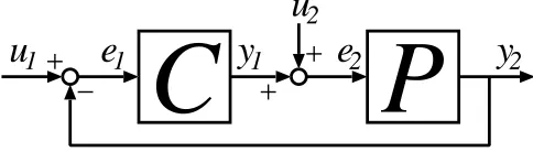
Fig. 1. Feedback systemΣ.
B. Feedback Stabilization Problem
The stabilization problem considered in this paper follows that of Sule in [11] and Mori and Abe in [10] who consider the feedback system Σ [3, Ch.5, Figure 5.1] as in Figure 1. For further details the reader is referred to [3], [10]. Through-out this paper, the plant we consider has m inputs and n
outputs, and its transfer matrix, which itself is also called simply a plant, is denoted by P and belongs toPn×m.
Definition 2: DefineFbadby
b
Fad = {(X, Y)∈ Fx×y× Fy×x|
det(Ix+XY)is a unit ofF, xandy are positive integers}.
For P ∈ Fn×m and C ∈ Fm×n, the matrix H(P, C) ∈ F(m+n)×(m+n) is defined by
H(P, C) =
(In+P C)−1 −P(Im+CP)−1 C(In+P C)−1 (Im+CP)−1
(1)
provided(P, C)∈Fbad. ThisH(P, C)is the transfer matrix
from[ut 1 ut2]
tto[et 1 et2]
tof the feedback systemΣ. If (i)
(P, C)∈ Fbad and (ii)H(P, C)∈ A(m+n)×(m+n), then we
say that the plant P is stabilizable, C stabilizes P, P is stabilized byC, andC is a stabilizing controller ofP.
In (1), there are two kind of inverse matrices,(In+P C)−1,
(Im+CP)−1. We can make them describe with only one
inverse matrix as follows:
H(P, C) =
I−P(Im+CP)−1C −P(Im+CP)−1
(Im+CP)−1C (Im+CP)−1
=
(In+P C)−1 −(In+P C)−1P C(In+P C)−1 Im−C(In+P C)−1P
.
It is known thatW(P, C) defined below is overAif and only ifH(P, C)is overA:
W(P, C) :=
C(In+P C)−1 −CP(Im+CP)−1 P C(In+P C)−1 P(Im+CP)−1
.
(2) This W(P, C) is the transfer matrix fromu1 and u2 to y1
andy2. Then, we have
H(P, C) =Im+n−F W(P, C),
where
F =
O In
−Im O
.
The matrixF is unimodular; in fact,
F−1=
O −Im In O
,
which is overA. Thus,W(P, C) can be expressed in terms ofF andH(P, C):
W(P, C) =F−1(Im
+n−H(P, C)).
Note 1: Instead of Definition 2, we can describe the defini-tion of the stabilify by usingW(P, C) rather thanH(P, C) as follows: For P ∈ Fn×m and C ∈ Fm×n, the matrix
W(P, C)∈ F(m+n)×(m+n) is as in (2) provided(P, C)∈
b
Fad. If (i)(P, C)∈Fbadand (ii)W(P, C)∈ A(m+n)×(m+n),
then we say that the plantP is stabilizable,C stabilizesP,
P is stabilized by C, andC is a stabilizing controller ofP.
It should be noted that when using “a stabilizing con-troller,” we do not guarantee the causality. However, in the classical case of the factorization approach, once we restrict ourselves to strictly proper plants, it is known that any stabilizing controller of strictly causal plant is causal (cf. Corollary 5.2.20 of [3], Theorem 4.1 of [4], and Propo-sition 6.2 of [10]). One can see, in fact, that many practical systems are strictly causal.
III. PARAMETRIZATION WITHOUTCOPRIME FACTORIZABILITY
Here we review the parametrization method without con-sidering the coprime factorizability[12], [13]. Let Hbe the set ofH(P, C)’s with all stabilizing controllersCof the plant
P. This set Hand all stabilizing controllers are obtained as in the following way.
LetH0 beH(P, C0), whereC0 is a stabilizing controller
ofP. LetΩ(Q)be a matrix defined as follows:
Ω(Q) := (H0−
In O O O
)Q (3)
×(H0−
O O O Im
) +H0
with a stable causal and square matrixQof size(m+n)×
(m+n). Using this matrixQ, we have the following theorem, the controller parametrization, as follows.
Theorem 1 ([12], [13]): The set of allH(P, C)’s with all stabilizing controllers is given as follows
H={Ω(Q)|Qis stable causal and Ω(Q)is nonsingular} (4) Furthermore, any stabilizing controller has the following form:
−[O Im] Ω(Q)−1In O
, (5)
provided thatΩ(Q)is nonsingular.
The parametrization above is given by a parameter ma-trixQwithout the coprime factorizability of the plant. This parametrization method is applicable to the stabilizable plant with no coprime factorization (of course, any plant which admits coprime factorization can also applied to).
The parameter matrix Q is of size (m+n)×(m+n). That is, in order to archive the parametrization, we need(m+
n)2parameters. On the other hand, the Youla-parametrization
needs onlymnparameters.
IAENG International Journal of Applied Mathematics, 44:4, IJAM_44_4_07
IV. MAINRESULT
The following is the parametrization of stabilizing con-trollers presented as a Youla-parametrization.
Theorem 2: (cf. Theorems 5.2.1 and 8.3.12 of [3]) Sup-pose that the plantP ∈ Pn×m is stabilizable. Suppose
fur-ther thatP admits right-/left-coprime factorizations overA ofP. Let (N, D)and (N ,e De) be right-/left-coprime factor-izations, respectively, overAofPand(Y0, X0)and(Ye0,Xe0)
be right-/left-coprime factorizations, respectively, overAof
C0, a stabilizing controller ofP, such that
e
Y0N+Xe0D=Im, N Ye 0+DXe 0=In.
Then all matricesX,Y,Xe,Ye over Asatisfying
e
Y N+XDe =Im, N Ye +DXe =In
are expressed as X = X0−N S, Y = Y0+DS, Xe =
e
X0−RNe andYe =Ye0+RDe forR andS inAm×n.
Further the set of all stabilizing controllers, denoted by
S(P), is given as
S(P) = {(Xe0−RNe)−1(Ye0+RDe)| R∈ Am×n
, Xe0−RNe is nonsingular}
= {(Y0+DS)(X0−N S)−1| S ∈ Am×n
, X0−N S is nonsingular}.
The “integral domain version” of Theorem 2 was already shown in Section 8 of [3] without the proof. Nevertheless, considering general commutative rings as the set of stable causal transfer functions, we need to give the proof because the proofs have some differences.
To make this paper as self-contained as we can, we inlucde some lemmas which has even appeared in some literatures already.
Lemma 1: (cf. 8.3.12 of [3]) Suppose that P ∈ Fn×m admits a right- (left-) coprime factorization andC∈ Fm×n is any stabilizing controller ofP. Then the stabilizing con-trollerC admits a left- (right-) coprime factorization.
Proof: Suppose thatP admits a right-coprime factoriza-tion. Let (N, D)be a right-coprime factorization overAof
P. Then existYe andXe overAsuch thatY Ne +XDe =Im. Let C be a stabilizing controller of P. Then H(P, C) is as follows:
H(P, C) = H(N D−1, C)
=
(In+N D−1C)−1
−N D−1(Im+CN D−1)−1 C(In+N D−1C)−1
(Im+CN D−1)−1
=
In−N(D+CN)−1C −N(D+CN)−1 D(D+CN)−1C D(D+CN)−1
.(6)
The matrix above is over A because C is a stabilizing controller. Now letS andT be
S = (D+CN)−1, T = (D+CN)−1C,
respectively. Then, S holds
S = (D+CN)−1
= Y Ne (D+CN)−1+XDe (D+CN)−1.
In the term Y Ne (D +CN)−1, Ye is over
A, and N(D+
CN)−1 is the negative of the (1,2)-block of (6). Further, in
the termXDe (D+CN)−1,Xe is overA, andD(D+CN)−1
is the (2,2)-block of (6). HenceS isA.
Analogously we show thatT is ofA. We now have
T = (D+CN)−1C
= Y Ne (D+CN)−1C+XDe (D+CN)−1C.
In the term Y Ne (D+CN)−1C,Ye is over
A, and N(D+
CN)−1C is a part of the (1,1)-block of (6). Further, in the
termXDe (D+CN)−1C,Xe is overA, andD(D+CN)−1C
is the (2,1)-block of (6). HenceT is alsoA.
In the following, we show that (T, S) is a left-coprime factorization over A of C. It is obvious C = ((D +
CN)−1)−1(D+CN)−1C = S−1T. Now consider SD+ T N, which is
SD+T N = (D+CN)−1D+ (D+CN)−1CN
= (D+CN)−1(D+CN) =Im.
Hence(T, S)is a left-coprime factorization overAofC. The discussion of the case whereP admits a left-coprime factorization overAcan be achieved entirely analogously.
Theorem 3: (cf. Theorem 4.1.60 of [3]) Suppose thatP∈ Fn×m and let (N, D) and (N ,e De) be a right- and a
left-coprime factorizations, respectively, over A. Suppose that matricesYe andXe over AsatisfyY Ne +XNe =Im.
Then there exist matricesY andX overAsuch that
e
X Ye −Ne De
D −Y
N X
=Im+n. (7)
Proof: BecauseNe andDe are left-coprime factorization over A ofP, there exist matrices Y1 and X1 over A such
thatN Ye 1+DXe 1=In. Define E =
e
X Ye −Ne De
.
Then
E
D −Y1 N X1
=
Im ∆
O In
, (8)
where∆ = −XYe 1+Y Xe 1 ∈ Am×n. Since the right hand
side of (8) is unimodular, so is E, whose inverse is
E−1 =
D −Y1 N X1
Im ∆
O In
−1
=
D −Y1 N X1
Im −∆
O In
=
D −(Y1+D∆) N X1−N∆
.
Then (7) is satisfied withY =Y1+D∆andX=X1−N∆.
The following corollary is the parallel result of Theorem 3. Corollary 1: Suppose that P ∈ Fn×m
and let (N, D) and (N ,e De) be a right- and a left-coprime factorizations, respectively, overA. Suppose that matricesY andX overA satisfyN Ye +DXe =In.
Then there exist matricesXe andYe over Asuch that (7) holds.
Theorem 4: (cf. Corollary 4.1.67 of [3]) Suppose that
P ∈ Fn×m and (N, D) and (N ,e De) be a right- and a
IAENG International Journal of Applied Mathematics, 44:4, IJAM_44_4_07
left-coprime factorizations, respectively, overAofP. Then for every matrices Ye, Xe, Y, and X over A such that
e
Y N+XDe =Im,N Ye +DXe =In, the matrices
U1=
e
X Ye −Ne De
, U2=
D −Y
N X
(9)
are unimodular. Moreover U−1
1 is a complementation of
[ Dt Nt]t, in thatU−1
1 is of the form
U−1 1 =
D G
N
(10)
for some matrixGover A. Analogously,U−1
2 is a
comple-mentation of[ −Ne De ], in thatU−1
2 is of the form
U−1 2 =
F
−Ne De
(11)
for some matrixF overA.
Proof: Using the right-coprimeness of (N, D) over overA, consider matricesYe andXe such thatY Ne +XDe =
Im. Then by Theorem 3, there exist matricesX andY over
Asuch that
e
X Ye −Ne De
D −Y
N X
=Im+n. (12)
LetU1 andU2 as in (9). Then by (12), they are unimodular.
Applying G = [−Yt Xt]t
, we have (10). Analogously, applyingF = [Ne Ye] we have (11).
Lemma 2: (cf. Lemma 3.1 of [4]) Suppose that P ∈ Fn×m andC ∈ Fm×n and let (N, D) be a right-coprime
factorization over A of P and (Y ,e Xe) a left-coprime fac-torization over A of C. Under these conditions, C is a stabilizing controller of P if and on ly if
∆1=Y Ne +XDe
is a unimodular ofA.
Proof: “If”: Suppose that∆1is a unimodular. Then∆ −1 1
is overA. First, sinceIm+CP =Xe−1∆
1D−1, we see that
det(Im+CP) = det(In+P C)is a nonzerodivisor. Next, we showH(P, C)is overA. By direct substitution inH(P, C), we have
H(P, C)
=
In−P(Im+CP)−1C −P(Im+CP)−1
(Im+CP)−1C (Im+CP)−1
=
In−P D∆−1
1 XCe −P D∆ −1 1 Xe D∆−1
1 XCe D∆
−1 1 Xe
=
In−N∆−1
1 Ye −N∆ −1 1 Xe D∆−1
1 Ye D∆ −1 1 Xe
. (13)
Because∆−1
1 is unimodular, thisH(P, C)is overA.
“Only If”: Suppose that C is a stabilizing controller of P. Thendet(Im+CP)6= 0 andH(P, C)is overA.
BecauseH(P, C)is overA. the following matrix, which is modified from (13), is also overA.
N∆−1
1 Ye N∆ −1 1 Xe D∆−1
1 Ye D∆ −1 1 Xe
. (14)
Recall that (N, D) is a right-coprime factorization over A ofP and (Y ,e Xe)a left-coprime factorization over AofC. Then there exist matricesA,B,R,S over Asuch that
e
AN+BDe =Im, Y Re +XSe =In.
By using these relation and (14), we have
∆−1
1 = [Ae Be]
N∆−1
1 Ye N∆ −1 1 Xe D∆−1
1 Ye D∆ −1 1 Xe
R S
. (15)
All matrices of the right hand side of (15) is overA. Hence ∆−1
1 is also overAand so ∆1 is unimodular.
Theorem 5: (cf. Corollary 5.1.30 of [3]) Suppose thatP∈ Fn×m
and let (N, D) and (N ,e De) be any right- and left-coprime factorization, respectively, overA. Suppose also that
Cadmits right- and left-coprime factorizations overA. Then the following are equivalent:
(i) C stabilizesP.
(ii) C has a left-coprime factorization(Y ,e Xe)over Awith
e
Y N+XDe =Im.
(iii) Chas a right-coprime factorization(Y, X)overAwith
e
N Y +N Xe =In.
Proof: (i)→(ii): Suppose that C stabilizesP. Suppose that (Ye1,Xe1) is a left-coprime factorization over A of C,
which may be different from(Y ,e Xe). Then by Lemma 2, ∆1=Ye1N+Xe1D
is a unimodular of A. By letting Ye = ∆−1
1 Ye1 and Xe =
∆−1
1 Xe1, we have (ii).
(ii)→(i): Suppose that C has a left-coprime factorization (Y ,e Xe)over A with Y Ne +XDe =Im. From this identity, we haveCP+Im=Xe−1D−1, which is nonsingular. Now H(P, C) is
H(P, C)
=
I−P(Im+CP)−1C −P(Im+CP)−1
(Im+CP)−1C (Im+CP)−1
=
I−P DXCe −P DXe DXCe DXe
=
In−NYe −NXe DYe DXe
, (16)
which is overA. ThusC stabiliziesP.
The equivalence of (i) and (iii) is proved analogously. Before presenting the generalization of Lemma 4.1.32 of [3], we should give a lemma which is a generalization of Corollary 4.1.26 of [3].
Lemma 3: (cf. Corollary 4.1.26 of [3]) Suppose P ∈ Fn×m
and that P = N D−1 = De−1Ne with the matrices N, D,N ,e De over A. Let F1 = [−Ne De] and F2 =
[Dt Nt]t
. Then the following are equivalent:
(i) N and D are right-coprime over A, and Ne and De
left-coprime overA.
(ii) There exist unimodular matrices U1 and U2 of the
formsU1= [Gt1 F1t] t
andU2= [F2 G2]for some
matricesG1 andG2 overA.
Proof: “(i)→(ii)”. By Theorem 3, there exist matrices
e
Y,Xe,Y, andX overAsuch that (7) holds. ThenU1is the
first matrix of the left hand side of (7). AlsoU2is the second
matrix of the left hand side of (7). That is, G1 = [Xe Ye]
andG2= [−Yt Xt]t.
“(ii)→(i)”. LetV beU−1
1 and decompose it into 4 blocks as
follows:
U−1 1 =V =
m n
m V11 V12 n V21 V22
.
IAENG International Journal of Applied Mathematics, 44:4, IJAM_44_4_07
Because U1V = Im+n, we have Ne(−V12) +DVe 22 = In.
Hence Ne andDe are left-coprime factorization overA. The right-coprimeness can be proved analogously. LetW
beU−1
2 and decompose it into 4 blocks as follows:
U−1
2 =W =
m n
m W11 W12 n W21 W22
.
Because W U2 = Im+n, we have W12N +W11D = Im.
Hence N andD are right-coprime factorization overA. Lemma 4: (cf. Lemma 4.1.32 of [3]) Suppose P ∈ Fn×m
. Let (N, D) and (N ,e De) be right-/left-coprime fac-torizations, respectively, overAofP. LetU1 andU2 be the
unimodular matrices of the form in (ii) of Lemma 3. Then the set of all matrices Ye ∈ Am×n and Xe ∈ Am×m with
e
Y N+XDe =Im is given by
[Xe Ye] = [Im R]U−1
2 , (17)
where R ∈ Am×n. Similarly the set of all matrices Y ∈ Am×n andX ∈ An×n withN Ye +DXe =In is given by
−Y X
=U−1 1
S In
, (18)
whereS∈ Am×n .
The proof of Lemma 4 is analogous to that of Lemma 4.1.32 of [3], in which Lemma 3 above is used instead of Corollary 4.1.26 of [3].
Proof of Lemma 4: It is necessary to show that (i) everyYe andXe of the form (17) satisfiesY Ne +N De =Im, and (ii) everyYe andXe satisfyY Ne +XDe =Imare of the form (17) for someR.
To prove (i), observe that U−1
2 U2=Im+n. Hence
e
Y N+XDe = [Xe Ye]
D N
= [Im R]U−1 2
D N
= [Im R]
Im O
= Im.
To prove (ii), suppose thatYe′ andXe′
satisfiesYe′
N+Xe′
D=
Im. DecomposeU2 as follows:
D G21 N G22
:=U2.
DefineR=Ye′
G22+Xe′G21. Then
[Xe′ e
Y′
]U2= [Xe′ Ye′]
D G21 N G22
= [Im R].
The proof concerningY andX can be given analogously. It is necessary to show that (i) everyY andX of the form (18) satisfiesN Ye +DXe =In, and (ii) everyY andX satisfy
e
N Y +DXe =In are of the form (18) for some S. To prove (i), observe that U−1
1 U1=Im+n. Hence
e
N Y +DXe = [−Ne De]
−Y X
= [−Ne De]U−1 1
S In
= [O In]
S In
= In.
To prove (ii), suppose thatY′ andX′
satisfiesN Ye ′ +DXe ′
=
In. DecomposeU1 as follows:
G11 G12 −Ne De
:=U1.
Then, defineS=−G11Y′+G12X′. Now we have
U1
−Y′
X′
=
G11 G12 −Ne De
−Y′
X′
=
S In
.
Now we can prove Theorem 2.
Proof of Theorem 2:
We prove the first representation only. The second one is proved analogously.
⊂. By Lamma 1, any stabilizing controller has both right-/right-coprime factorizations overA.
It is shown in Theorem 5 thatC is stabilized byP if and only ifChas a left-coprime factorization(Y ,e Xe)overAsuch thatY Ne +XDe =Im. Now consider another left-coprime factorization(Ye′
,Xe′
)such that
e
Y′
N+Xe′
N =Im (19)
in the unknown matricesYe′ andXe′
. Then, again by Theo-rem 5,CstabilizesPif and only ifCis of the formXe′−1Ye′ forXe′
∈ Am×mand Ye′
∈ Am×n such that (19) holds and
e
X′
is nonsingular. From Theorem 4, the matrix
U1=
e
X Ye −Ne De
(20)
is unimodular, and moreoverU−1
1 is of the form
U−1 1 =
D G
N
,
whereGis a matrix over overA. By Lemma 4, we have all solutions for(Ye′
,Xe′
)of (19) are of the form [Xe′ e
Y′
] = [I R]U1= [Xe−RNe Ye+RDe]
for someR∈ Am×n.
V. EXAMPLE
Let us consider Anantharam’s example. Anantharam [7] considered the caseA=Z[√−5] ={u+v√−5|u, v∈Z}, whereZdenotes the set of integers (This ring [14, pp.134– 135] is isomorphic toZ[x]/(x2+5)and is an integral domain
but not a unique factorization domain. In fact,6∈Z[√−5] has two factorizations,2·3 and (1 +√−5)·(1−√−5)). He showed that a single-input single-output plant p = (1 +√−5)/2 does not admit a coprime factorization but is stabilizable and c = (1−√−5)/(−2) is a stabilizing controller.
Let us considerp= 5/2, then we have coprime factoriza-tion
y·5 +x·2 = 1,
where y = 1 and x = −2. Thus the set of all stbilizing controllers is given as
{ (y+ 2r)/(x−5r)| r∈ A }.
IAENG International Journal of Applied Mathematics, 44:4, IJAM_44_4_07
VI. CONCLUSIONS
In this paper, we consider the factorization approach to control systems with plants admitting coprime factoriza-tions and with the set of stable causal transfer funcfactoriza-tions being a general commutative ring. We have shown that the parametrization of stabilizing controllers is still achieved by the Youla-parametrization.
REFERENCES
[1] C. Desoer, R. Liu, J. Murray, and R. Saeks, “Feedback system design: The fractional representation approach to analysis and synthesis,” IEEE
Trans. Automat. Contr., vol. AC-25, pp. 399–412, 1980.
[2] V. Raman and R. Liu, “A necessary and sufficient condition for feedback stabilization in a factor ring,” IEEE Trans. Automat. Contr., vol. AC-29, pp. 941–943, 1984.
[3] M. Vidyasagar, Control System Synthesis: A Factorization Approach. Cambridge, MA: MIT Press, 1985.
[4] M. Vidyasagar, H. Schneider, and B. Francis, “Algebraic and topolog-ical aspects of feedback stabilization,” IEEE Trans. Automat. Contr., vol. AC-27, pp. 880–894, 1982.
[5] D. Youla, H. Jabr, and J. Bongiorno, Jr., “Modern Wiener-Hopf design of optimal controllers, Part II: The multivariable case,” IEEE Trans.
Automat. Contr., vol. AC-21, pp. 319–338, 1976.
[6] K. Mori, “General parameterization of stabilizing controllers with coprime factorizations,” Lecture Notes in Engineering and Computer
Science: Proceedings of The World Congress on Engineering 2014, 2-4 July, 2014, London, U.K., pp. 755–758.
[7] V. Anantharam, “On stabilization and the existence of coprime factor-izations,” IEEE Trans. Automat. Contr., vol. AC-30, pp. 1030–1031, 1985.
[8] K. Mori, “Feedback stabilization over commutative rings with no right-/left-coprime factorizations,” in CDC′99, 1999, pp. 973–975.
[9] ——, “Parameterization of stabilizing controllers with either right- or left-coprime factorization,” IEEE Trans. Automat. Contr., pp. 1763– 1767, Oct. 2002.
[10] K. Mori and K. Abe, “Feedback stabilization over commutative rings: Further study of coordinate-free approach,” SIAM J. Control and
Optim., vol. 39, no. 6, pp. 1952–1973, 2001.
[11] V. Sule, “Feedback stabilization over commutative rings: The matrix case,” SIAM J. Control and Optim., vol. 32, no. 6, pp. 1675–1695, 1994.
[12] K. Mori, “Parameterization of stabilizing controllers over commutative rings with application to multidimensional systems,” IEEE Trans.
Circuits and Syst. I, vol. 49, pp. 743–752, 2002.
[13] ——, “Elementary proof of controller parametrization without coprime factorizability,” IEEE Trans. Automat. Contr., vol. AC-49, pp. 589– 592, 2004.
[14] L. Sigler, Algebra. New York, NY: Springer-Verlag, 1976.