Abstract—Water scarcity remain a major challenge facing many countries around the world. These water challenges results to seeking other possible water alternatives techniques to save available water. Greywater reuse is one such alternative to save water if it can be treated successfully to meet greywater standards for reuse. However, within the usability of greywater at the core is the ability to monitor its quality during treatment that will meet the required standard of water for reuse particularly when water reuse alternatives are considered. The aim of the this paper is to demonstrate beyond the potential usability of the Horizontal Roughing Filter (HRF) which was identified as a possible greywater reuse treatment option/technology while monitoring its performance and effluent greywater quality using principal component approach and principal component regression techniques in HRF as a tool of provision of possible practical solution in community facing water challenges. The study was conducted using a pilot scale HRF to treat informal settlement greywater in the study area in Durban Umlazi, Southern Africa. Results showed that HRF was able to achieve removal efficiency of turbidity in greywater effluent above 90% at a filtration ate of 0.3 m/h and 60% chemical oxygen demand (COD). The predictor variables were temperature, COD, conductivity, total solids and pH. The principal component regression was more robust to identify performance relationship in the data better than multiple linear regression.
Index Terms—Principal component regression, horizontal roughing filter, principal component analyses, greywater, informal settlement
I. INTRODUCTION
u
ntreated greywater generated is one such available immense resource that could potentially find significant applications in countries facing water scarcity with application of simple treatment technology to treat greywater.Greywater is wastewater generated from household applications such as washing, bathing and laundry without input from toilets [1] and [2]. However, water monitoring quality techniques and HRF monitoring techniques become essential in any water treatment process. According to [3], rivers, drinking water, fisheries, agricultural sector, industry and energy productions all require and depend on quality. The water quality mainly comprises of physical, chemical and biological compositions [4]. For instance, the level of nutrients is a function of biological activity such as NO3 or
NH4 and physical properties that affects nutrients
transportation mechanism. All these water quality factors must be analyzed in the process of modelling any water quality. The measured effluent greywater parameters and its association /impact in water must be analyzed. Therefore the multivariate algorithm techniques of water parameters such as multiple linear regression (MLR), principal component analysis (PCA), partial least squares (PLS) analysis can be applied to understand the underlying structures and identification of possible influential factors in water treatment in the data, association, correlation in data including predictions using measured covariates of the model for better solution in interpretation of complex water data matrices [5].
Over the years, multivariate regression techniques and factor analyses have been extensively used for water quality monitoring purposes and for interpretation of water matrices correlation. [6] used principal components analyses to study water quality variations in the reservoir in Saddam dam. In this study, Algae, electrical conductivity and total solids were the only three parameters that were identified and associated with the seasonal variability in water quality. [7] also conducted a study for water quality assessment factors in Porsuk Tributary-Sakarya river basin using PCA and several parameters were identified a source of variation in water quality. In south West India, [8] conducted a study on water quality from the Cochin coast and developed a statistical model using PCA. The study was intended to identify relationship on physicochemical variables in coastal water.
[9] conducted a study using PCA and multiple regression analyses in Northern Thailand. The aim was to estimate the suspended sediment yield in river basin. In this study, six principal components were identified with 86.7% variance of identified variables and sediment yield predictors were found to be land use, rainfall distribution, basin size and
Performance of Horizontal Roughing Filter
Using Principal Component Regression and
Multiple Linear Regression Treating Informal
Settlement Greywater
1,2
S. Mtsweni,
1B.F. Bakare and
2S. Rathilal
Manuscript received May 15, 2017; revised July 12, 2017. 1. Department of Chemical Engineering,Mangosuthu University of Technology, 511 Mangosuthu Highway, Durban South Africa. 4031. Phone: +27319077447; fax: +27319077307; email: [email protected]
steepness and channeling network characteristics. [10] used principal component regression, artificial neural network and hybrid models for the prediction of phytoplankton abundance in Macau storage reservoir. In this study, the artificial neural network better performed than both principal component regression and hybrid models.
Currently most of the available studies have mainly focused into the feasibility of HRF to show its ability as a potential cheap available treatment technology in removal of physical, biological and chemical pollutants in greywater. Most of these studies were conducted based on synthetic wastewater and few on natural wastewater. Another studies have focused on the HRF modelling using existing performance modelling techniques to study flow mechanism within the HRF, particle size effect and water quality prediction using neural network [11-17]. This study focuses largely on the greywater reuse in horizontal roughing filter and greywater quality monitoring modelling techniques in a horizontal roughing filter for the informal settlement collected greywater for the provision of alternatives of discarded greywater in this informal settlement.
[image:2.595.307.545.51.776.2]
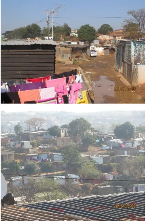
The study area is situated at the outskirt of Southern part of Durban - Umlazi. The area is a densely populated with informal settlements. It is a non-sewered area with limited number of basic social needs such as the waste management infrastructure, schools and health services as shown in Figure 1&2 below. The area was identified and selected for a practical representation of greywater challenges.
Figure 1: Study area informal settlements Figure 2: Greywater runoffs in the study area
[image:2.595.46.289.407.776.2]II. MATERIALSANDMETHODS
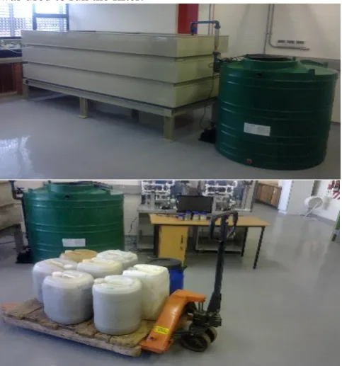
[image:3.595.47.289.286.545.2]The study framework involved data collection, principal component analysis, multiple regression analysis and principal component regression. At first instance, greywater collection (three times a week) for a period of three months from the informal settlement of the study area was the primary focus. For each run, 420 litres the collected greywater samples were transported from the community to the Mangosuthu University of Technology, Chemical Engineering research laboratory for experimental work using a constructed pilot scale HRF with 3 m length (Figure 3 below). Quartzite gravel was selected and used as a filter media in the roughing filter. The gravel sizes were: 15 - 13.2 mm in 1st compartment; 13.2 - 9.5 mm in 2nd compartment and 9.5 - 6.7 mm in 3rd compartment. The operating mode of the horizontal roughing filter system was based on the batch feeding mode. After manually filling the feed tank with 420 litres required for the single batch operation, a predetermine filtration rate between 0.3 m/h was used to run the filter.
Figure 3: HRF and collected greywater samples for treatment
All water analyses were performed according to the standard methods for the wastewater analyses [18]. These included total dissolved solids (TDS), electrical conductivity (EC), chemical oxygen demand (COD), pH, turbidity and biological oxygen demand (BOD5). The quality parameters were selected based on their potential social impact and implications on human health conditions and environmental pollution contribution effects.
The data reduction technique - principal component analysis was applied in the effluent greywater from the HRF. This was done to identify the significant influential factors to the filter efficiency and the level of multicollinearity in the independent variables for the subsequent analyses of data and development of multiple linear regression. The following steps were performed during PCA:data
assessment by performing Kaiser-Meyer-Olkin (KMO) with a score of 0.5 obtained and the Bartlett’s test of sphericity was obtained to be significant. Correlation coefficients in correlation matrix step were found to meet the criteria of greater than or equal to 0.30 as suggested by [19]. To identify principal components, the Varimax rotation was used to identify subset of variables in each principal component identified. The eigenvalues criterion of 1.0 or above was used with a scree plot to retain significant components.
Multiple linear regression was applied in effluent greywater relating filter efficiency and all physical and chemical parameters of the effluent greywater. This was done to identify variable inflation factor and multicollinearity amongst variables. The filter efficiency was regressed on dominant factors identified and obtained through principal component analysis in the form of equation 1:
)
1
...(
....
2 2 1 1
0
x
x
px
p
, where Y,represents filter efficiency,
x
1,x
2, …,x
p are thepredictor variables or the factors influencing filter performance/efficiency and
0,
1,
2,…,
p areconstants obtained through multiple linear regression analysis.
III. RESULTSANDDISCUSSIONS
The experimental data used for subsequently statistical analyses was obtained from experimental runs conducted in the horizontal roughing filter. The filter was treating 420 litres of mixed greywater per batch run collected from the informal settlement in Umlazi in Durban. Several greywater parameters per each batch run were analyzed for the measurement of the horizontal roughing filter performance analyses. The variables were measured in order to better understand the level of removal of pollutants in greywater effluent from the horizontal roughing filter were conductivity, pH, temperature, total solids and COD. These parameters were specifically selected for analyses in order to predict the horizontal roughing filter performance based on physical and chemical pollutants removal in effluent greywater from the horizontal roughing filter. All experiments were conducted in 0.3 m/h filtration rates in three compartment roughing filter. There were five predictor variables used for the multivariable linear regression. Conductivity, turbidity, pH, COD and total solids. The average values for conductivity, temperature and total solids were 302 μS/cm, 22 °C and 41 mg/l respectively for a percentage removal of 95% turbidity. The average COD value was 1161 mg/l. Both physical and chemical pollutants were found to be significant different by statistical analysis of analyses of variance (ANOVA) test and t-test at a significant level, p-value below 0.05.
criterion was set to be 3 or -3 for any z-score value and the Cook’s distance test with p < 0.01 was used as a criterion for multivariate outlier. The data was inspected for normality distribution using normal Q-Q plot and scatter plot for confirmation if the data meets normal distribution assumptions and validity of application of normal distribution statistics. The data was found to be fairly within the straight line confirming that the residuals are from the normal distribution population. The adjusted R-square of 0.9 for multiple linear regression model as obtained which is an indication of variance in the dependent variable, the turbidity, explained by the physical and chemical predictor variables to be 91% and the variance inflation factor (VIF) was found to be below a value of 10 which is the normal acceptable level. The highest standardized coefficient value of the multiple linear regression was obtained to be 0.72 which was the coefficient value for total solids.
Principal component regression
The original data was normalized for each of the five measured parameters by subtracting the calculated mean and dividing with the calculated standard deviation. This was done for all variables in the original data for conductivity, turbidity, total solids, COD and pH. These was done to linearly transform the different measured scale of unit in these variables and to minimize the dominance of larger scale units thus standardizing all units to a range between -10 to -10. The standardization was
z
(
x
x
average)
/
sd
where
x
x
average is the observed value, mean valuerespectively and
sd
is the standard deviation of the data corresponding with each parameter standardized. The dependent variable was centered by calculating the mean of the data and the mean value was subtracted in each observed data point byy
y
mean, wherey
andy
mean represent dependent variable and mean value of the dependent variable.The Kaiser-Meyer-Olkin (KMO) test for assessment of validity of PCA application and sample adequacy was conducted and was found to be 0.5. The Bartlett test of sphericity was significant with p value less than < 0.01. This indicates non-orthogonality amongst variables. The correlation matrix via principal component analyses was then computed and obtained and the and as well as eigenvalues and eigenvectors. Varimax rotation technique was applied to assess overlapping of the original variables across each identified principal components.
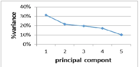
The water quality parameters through matrix of rotated Varimax were grouped in to two principal components which explained the cumulative percentage of 95% of the total variance. The covariance matrix of for the standardized data matrix were computed and the eigenvectors and eigenvalues which were obtained from the PCA analysis were used to develop principal component regression. The scree plot was developed showing the percentage variance of the extracted component as shown below in Figure 4. The first principal component explained 31% variance and
74% variance explained by the first three principal components and eigenvalues above 1.0.
Figure 4: Scree plot percentage variance of the extracted principal components
All components were considered in the data analyses for principal component egression and the modified data was obtained using
z
matrix
x
(nxp)
(pxq) wherez
matrix, isthe modified standardized data matrix,
x
(nxp) is the originalmatrix of the standardized data of the predictor variables and
(pxq)is the matrix of the eigenvectors obtained fromprincipal component analysis corresponding with PCA values. The product of standardized
variable which is the dependent variable and the transpose ofz
matrix which is [image:4.595.306.547.84.200.2]denoted as
z
matrix was obtained and modified. The final new data matrix values are presented in Table 1 below.Table 1:
z
matrix-108.80 -341.52 -153.04
60.30 103.84
The inverse matrix, (
z
z
matrix)1 was obtained usingmathematical relations from the calculated
z
matrix and z
matrix, the transpose matrix of the
z
matrix. The values of the inverse matrix results are tabulated below in Table 2.Table 2: Inverse matrix of modified data
The regression coefficients were then obtained using the (
z
z
matrix)1
, the standardized / centered
dependent values with the product of
z
matrix. The product of inverse matrix and the product of
z
matrix were used0.02 0.00 0.00 0.00 0.00
0.00 0.02 0.00 0.00 0.00
0.00 0.00 0.03 0.00 0.00
0.00 0.00 0.00 0.03 0.00
0.00 0.00 0.00 0.00 0.05
[image:4.595.306.549.623.707.2]to obtain the values of the regression coefficients and the coefficient values are shown in Table 3 below.
Table 3: PCR coefficients values -1.78
-8.07 -3.99 1.80
5.24
The final principal component regression is
5 4 3 2 1 24 . 5 80 . 1 99 . 3 07 . 8 78 . 1
c
c
c
c
c
Where
c
i is the principal component regression corresponding withi
1
,
2
,
3
,
4
,
5
= 1,2,3,4, 5 the value numbers of the principal components. Y is the dependent standardized variable. The R-square value was calculated to be 0.91.IV. CONCLUSIONS
In multiple linear regression, there were five predictor variables included in multiple linear regression. The multivariable regression equation was able to relates predictor variables of the effluent greywater from the roughing filter with the adjusted R-square value of 0.91. Few principal component regression models were developed but the final developed principal component regression model obtained was with the R-square value of 0.915 for 100% of explained variance for all principal components. The principal component regression model demonstrated a better ability to estimate greywater quality and a better greywater turbidity model through principal component regression.
REFERENCES
[1] LUDWIG, A. (2006) The new create an oasis with greywater: oasis design, Santa Barbara, California.
[2] JEFFERSON, B., PALMER, A., JEFFREY, P., STUETZ, R. AND JUDD, S. (2004) Greywater characterization and its impact on the selection and operation of technologies for urban reuse, Water Science and Technology, 50(2):157–164.
[3] ISCEN C.F., EMIROGLU O., ILHAN S., ARSLAN N., YILMAZ V. AND AHISKA S. (2008), Application of multivariate statistical techniques in the assessment of surface water quality in Uluabat Lake, Turkey. Environmental monitoring and assessment, 144(1-3): 269-276.
[4] MUSTAPHA, A., AND ADO A. (2012) Application of Principal Component Analysis & Multiple Regression Models in Surface Water Quality Assessment. Journal of Environment and Earth Science, 2(2):16-23.
[5] BOYACIOGLU H., BOYACIOGLU, H. AND GUNDUZ, O. (2005) Application of factor analysis in assessment of surface water quality in Buyuk Menderes River Basin, European Water Journal, 9(10): 43-49.
[6] SHIHAB, S. (1993) Application of Multivariate Method in the Interpretation of Water Quality Monitoring Data of Saddam Dam Reservoir, Confidential 13.
[7] MAZLUM, N., OZER, A. AND MAZLUM, S. (1996) Interpretation of Water Quality Data by Principal Components Analysis”, Journal of Engineering and Environmental Science, 23:19-26.
[8] IYER, C.S., SINDHU, M., KULKARNI, S.G., TAMBE, S.S AND KULKARNI, B.D. (2003)
Statistical analysis of the physico-chemical data on the coastal water of Cochin, Journal of Environmental Monitoring, 2(5): 324-327.
[9] WUTTICHAIKITCHAROEN, P. AND BABEL, M.S. (2014) Principal Component and Multiple Regression Analyses for the Estimation of Suspended Sediment
Yield in Ungauged Basins of Northern Thailand. Water, 6(8): 2412-2435.
[10] IEK IN IEONG, INCHIO LOU, WAI KIN UNG AND KAI MENG MOK (2015) Using principal component regression, artificial neural network, and hybrid models for predicting phytoplankton abundance in Macau storage reservoir, Environ model assess, 20:355-365.
[11] WEGELIN, M. (1996) Surface water treatment by roughing filters - A design, construction and operation manual, SANDEC Report No. 2/96, Dubendorf, Switzerland.
[12] BOLLER, M. (1993) Filter mechanisms in roughing filters. Journal of Water Supply Research and Technology–Aqua, 42(3):174-85.
[13] COLLINS, M.R., COLE, J.O. AND PARIS, D.B. (1994a) Assessing roughing filtration design variables. Water Supply, 12:1-2.
[14] WEGELIN, M. (1986) Horizontal flow roughing filtration (HRF), design, construction and operation manual, IRCWD Report No. 06/86, Zurich, Switzerland.
[15] MUKHOPADHAY, B., MUJUMDER, M., BARMAN, R.N., ROY, P.K. AND MAZUMDAR, A. (2009) Verification of filter efficiency of horizontal roughing filter by Wegelin’s design criteria and artificial neural network. Drinking Water Engineering and Science Discussions, 2(4):21-27.
[16] LEBCIR, R. (1992) Factors controlling the performance of horizontal flow roughing filters. Ph.D thesis, the University of Newcastle upon Tyne, UK, 1992.
[17] IVES, K. J. AND SHOLJI, I. (1965) Research on variables affecting filtration. Journal of Sanitary Engineering Division, ASCE, 91(SA4): 1-18.
[18] AMERICAN PUBLIC HEALTH ASSOCIATION, APHA. (1998) Standards methods for the examination of water and wastewater, 20th edition. American Water Works Association and Water Environmental Federation, Washington, DC.
[19] TABACHNICK, B.G.; FIDELL, L.S. (2001) Using Multivariate Statistics; Harper Collins: New York, USA.