Determinants of Estimated Measurement for Malaria Mortality using Modified State Estimation Model in a Case of a Developing Country

(1)

Determinants of Estimated Measurement for

Malaria Mortality using Modified State Estimation

Model in a Case of a Developing Country

S. L. Braide, D.C. Idoniboyeobu

Abstract— This paper considers careful selective monitoring of basic human health status is a vital consideration to the well being of man and society, which has been providing the data needed for the effective planning and management for daily activities of human endeavour for purpose of social and economic developments. Many researchers and scholars has contributed to the prediction of incidence and recovery rate for malaria mortality. This technical paper, modified state estimation model for malaria mortality in a developing country which is based on the mathematical model principles of: matrix formulation techniques, weighted sum of squares of errors techniques, chi-square distribution techniques, instrument measurement technique (sphygmomanometer etc) were manipulated and structured for this study case. Four (4) measurements were collected from different geographical locations for patients with malaria endemic cases. The physical measurements were implemented into the developed modified equations for purpose of estimating the physicians measurement on the view to check error to be classified as bad data measurement. The results obtained shows bad data measurement, which may be attributed to: poor instrument calibration problems, the surrounding circumstance of the patients, aging of the instrument, sensitivity, temperature/humidity of instruments may be responsible. The model is validated with calculated value of the objective function (f) and chi-square distributions, 2 degree of freedom with 99% significance level of confidence with suspected error measurements. The matrix formulation in state-estimation model is also coded in matrix laboratory environment for validation which gives similar results, the calculated value of the state variable



x₁,x₂



: 8.5225&13.235 which is represented and coded as V in the matlab environment, indicating low pulse rate of the measured body state blood pressure (Bp), that required attension to be true for acceptance.

Index Terms— Measurement, Matrix formulations, malaria, mortality, state-estimates, distribution.

I. INTRODUCTION

Improved State Estimation Model Techniques and Governing Equations

he analysis and investigation of basic human body diagnosis uses the vital statistics variables of physical measurement because it deals with scientific application to the life history of communities and nation. That is historical development which is a function of human society can be numerically be expressed qualitatively or quantitatively. The purpose of this study is to find out the changing composition of communities or nations with reference to sex, age, education, economic and civic status which is considered under study [8].

S. L. Braide, Department of Electrical/Computer Engineering, Rivers State University, Nkpolu Oroworukwo, Port Harcourt, Nigeria,

[email protected]; [email protected]

D.C. Idoniboyeobu, Department of Electrical/Computer Engineering Rivers State University, Nkpolu Oroworukwo, Port Harcourt

Evidently the state estimation model considered the numerical records of marriage, births, sickness and deaths by which the health and growth of community may be studied. The vital statistics variable provides the results of the biometry which deals with data and the laws of human mortality, morbidity and demography [1].

This technical contents considered the data or the laws which explain the phenomenon of birth, deaths, health and longevity, composition and concentration etc.

This study can also be extended to solve information particularly on fertility, mortality, maternity, urban density which is indispensable for planning and evaluation of the schemes of health, family planning and other vital amenities for purpose of efficient planning, evaluation and analysis of various economic and social policies [4].

Importantly, data collected on life expectancy at various age levels is helpful in actual calculations of risk on life policies, this means that life table called the biometer of public health and longivity helps in fixing the life insurance premium rates at various age level.

The modified state estimation model described the estimation strategy using different mathematical matrics operations to estimates the physical measurements carried out by a physician/medical doctors, on the view to determine the estimated physical measurements for malaria mortality in a developing countries, the question is how true? is the physical measurement taken by the medical doctor for purpose of placing drug dispensation and administration evidently, research studies has provided with results the measurement equations characterizing the meter readings with the view to the addition of error terms to the system model for purpose of validating physical measurement by medical practioners [10].

Several measurement instruments and devices are used in the measurements of vital statistics variable (state-variables) of the human life expectancy. We have the sphygmomanotreter (device that measures blood pressure) thermometer (device that measures temperature), (blood sugar level), (plasmodium viviax: parasite for malaria) etc [11].

(2)

accuracy are exceeded because of noise the true values of physical quantities are never known and we have to consider how to calculate the best possible estimates of the unknown quantities [9].

Incidentally, the techniques of least square is often used to best fit measurement data relating to two or more quantities. However modified equations are developed and formulated to characterize measurements of the physical data collected or acquired from patients for purpose of analysis with the integration of errors terms in the system model. The best estimates are choosen which minimizes the weighted sum of squares of the measurement errors [12].

II. BACKGROUND OF STUDY

State estimation techniques is the process of determining a set of values for a set of unknown systems (Engineering systems, human being systems, medical systems, biological systems, machine/instruments system etc). State variables are based on certain criterion making use of physical measurements made which are not precise due to inherent error associated with controllers/transducers and sometimes creates redundancy of measurement that does not require assessment of the true-value of the systems state variables [3]. Statistical methods are also used to estimate the true value of the system state variables with the minimum number of variables required to analyse the system in all aspects. The measurements taken by a medical practitioner are required to meet the basic records for a given circumstances intended to address particularly to the engineering systems, medical system, biological systems and related systems in order to provide good quality of reliable physical measurements for system variables [6]. Evidently, the necessary conditions for vital statistics variables analysis for administering drugs dispension to patients ensure and declared measurements records conformity to calculation of the measuring instruments, precision and tolerance for purpose of standard practice for world health organization (WHO) [5].

Importantly, if the measurement instruments introduces errors while undertaking details information variables statistics about patients status, this may results into wrong presentation of recorded data required for prescription/dispensing of drugs this will eventually results into gradual breakdown of human body system, immunity, antibodies vital tissues and sensitive organs like liver, kidney etc in a colossal decay condition that may leads to early mortality for associated emergence of infected and transmitted diseases [2].

Essentially for purpose of good working condition of human lives, standard practice for healthy living, is strongly monitored in order to regularly checked for recalibration of measuring instruments, for purpose of high precision, tolerance and accuracy [6].

III. MATERIALS AND METHOD

Model Formulation of Modified State Estimation Equations

The measurement set used by medical practioners consists of thermometer reading (z₁), sphygmomanometer (z₂), Blood-sugar level (z₃) and plasmodiums vivax parasite

transmission measurement (z₄) etc. Where z₁, z₂, z₃, andz₄, are mathematical measurement parameter sowing to the physical measurements/quantities respectively.

Similarly, the symbol x represents physical quantities being estimated.

Then the measurement equations that is characterizing the meter readings/measured terms are found by adding error terms (e) to the system model as:

e Hx

Z   (1)

Z: Measurement variables H: rectangular matrice operations.

x: State variables (the physical quantities being estimated). e: errors term

hx: True values of system model

The numerical coefficient are determined by the human body circulatory components and the error terms

e

1

,

e

2

,

e

3

and

e

4which represents errors in measurement

z

1

,

z

2

,

z

3

and

z

₄ respectively.

If the errors terms



e

₁

,

e

₂

,

e

₃

,

e

₄



are zero, then it is an ideal condition which mean that the meter reading of the physical measurement taken by the vital statistics variable of the patients are exact and true measurements

 

z

,which gives exact values of

x

₁and

x

₂ of

x

ˆ

₁and

ˆ

x

₂which could be determined.

From the relationship of equation (1) it can be obtained as:

1 , 1 1 2 12 1 11

1

h

x

h

x

e

z

e

z









_true



(2)

2 , 2 2 2 22 1 21

2

h

x

h

x

e

z

e

z









_true



(3)

3 , 3 3 2 32 1 31

3

h

x

h

x

e

z

e

z









_true



(4)

1 , 4 4 2 42 1 41

4

h

x

h

x

e

z

e

z









_true



(5)

Where;

Z

;

_truetrue: True value of the measured quantity z_j Reformulating equation (2) – (5) into vector form to obtained as;























































4 3 2 1

4 3 2 , 1

4 3 2 1

z

e

true true true true

–













42 41

32 31

22 21

12 11

h













2 1

x

(6)

(3)

Hx

z

e





_true





(7)

Which represents the error term between the actual measurement (z) and the true (but unknown) values

Hx

z

_true  of the measurement quantities. The true values of x₁ and x₂ cannot be determined but we can calculate the estimates

x

ˆ

₁ and

x

ˆ

₂.

Substituting these estimates (

x

ˆ

₁ and

x

ˆ

₂) into equation (6) gives the estimated values of the errors in the form as:













4 3 2 1

ˆ

e

=













4 3 2 1

z

–













42 41 32 31 22 21 12 11

h













2 1

ˆ

x

(8)

The quantitie are estimates of the corresponding quantities.

The vector, eˆ which represents the differences between the actual measurement (z) and their estimated values

 

zˆ  Hxˆ

, thus in compact form is given as:



x



H

e

x

H

z

e

ˆ





ˆ





ˆ





ˆ



(9)

The criterion for calculating the estimates

x

ˆ

₁ and

x

ˆ

₂can be determined as:





T

e

ˆ



ˆ

₁

ˆ

₂

ˆ

₃

ˆ

₄ (10)

and





T

z

ˆ



ˆ

₁

ˆ

₂

ˆ

₃

ˆ

₄ (11)

Equation (10) and (11) have to be computed for purpose of estimation analysis.

The techniques can be used to describe algebraic sum of errors to minimize positive and negative operations which may not be acceptable.

However, it is preferable to minimize the direct sum of squares of errors.

To ensure that measurement from meters or data collected of known greater accuracy are considered more favorably than less accurate measurements instrument/device, that is in each term the sum of squares is multiplied by an appropriate weighting factor (w) to give the objective function as: 2 4 4 2 3 3 2 2 2 2 1 1 4 1 2

e

w

e

w

e

w

e

w

e

w

f

j j

j











(12)

We select the best estimates of the state variables as those values

x

ˆ

₁ and

x

ˆ

₂ which cause the objectives functions (f) to take on its minimum value.

In accordance to the application of necessary conditions for minimizing function (f), the estimates

x

ˆ

₁ and

x

ˆ

₂ are those values of

x

₁ and

x

₂ which satisfy the equations as;

0

2

ˆ 1 4 4 4 1 3 3 3 2 2 2 2 1 1 1 1 ˆ 1

































x x

x

e

w

x

e

w

x

e

w

x

e

w

x

f

(13) Similarly,

0

2

ˆ 2 4 4 4 2 3 3 3 2 2 2 2 2 1 1 1 ˆ 2

































x x

x

e

w

x

e

w

x

e

w

x

e

w

x

f

(14)

That is, the notation: _ˆ



0

x which, indicates that the

equations have to be evaluated from the state estimates





T

x

ˆ



ˆ

₁

ˆ

₂ since the true values for the states variable are not known.

The unknown actual error (ej) are then replaced by estimated errors

e

ˆ

j which can be calculated once the true estimate

x

ˆ

i are known.

Equation (14) and (15) can be represented in vector form as:

                                                         0 0 ˆ 4 3 2 1 4 3 2 1 2 4 1 4 2 3 1 3 2 2 1 2 2 1 1 1 e e e e w w w w x x e x e x e x e x e x e x e x e x x x x x x x x x x x x (15)

Where w is the diagonal matrix of weighting factor which have special significance to the accuracy of measurement. The partial derivatives for substitution in equation 15 are found from equations (2) through (5) to be constant given by the elements (H) given as:

                                     0 0 ˆ ˆ ˆ ˆ 4 3 2 1 4 3 2 1 42 41 32 31 22 21 12 11 e e e e w w w w h h h h h h h h x x x x x x x x x x x x (16)

Using the operation of the compact notation process of equation (9) can be applied to also represent equation (17) as:



ˆ



0

ˆ



H

W

z



H

x



e

W

H

T T (17)

Multiplying through this equation (17) and solving for the estimates (

x

ˆ

) as:



H

WH



H

WZ

G

H

WZ

x

T T

G

T 1 1

2 1

ˆ































(18)

(4)





1

1 

 _

WH H

G T (19)

Which is also symmetrical in the mathematical operations. Essentially, the weighted least-squares procedure are required to estimates

x

ˆ

_i how close to the true value

x

_i of the state variables,

The expression for the difference _

  



 _

i x i

x is found my

substituting for;

Z=Hx + e to obtain as: (20)



Hx e



G



H WH



x G H We W

H G

x T

G T

T 1 1

1

ˆ_  _ _  _ 

  

(21)It

is an important consideration to check the useful operation of the dimensions of each term in the matrix product of equation (21) which is an important idea for developing properties of the weighted least-square estimations. In this analysis we have the matrix operation:

G

1

H

T

W

which as an overall operation of row × column dimensions of 2×4, which means that any one or more of the four errors



e

1

e

2

e

3

e

4



can influence the difference between each

state estimates.

The weighted least squares calculations spread the effects of the errors in any one measurements to some or all other estimates the characteristics is the basis for detecting bad data measurement.

In a similar manner we can compare the calculated values of

x

H

z

ˆ



ˆ

of the measured quantities with their actual measurements (z) by substituting for

x

ˆ



x

from equation (21) into equation (7) to obtain as:





e

T e

T

W

H

HG

I

W

H

HG

e

z

e

ˆ





ˆ





1





1 (22)

Where; I: unit or identity matrix. Statistical Analysis, Errors and Estimates

In reality we know absolutely true state of a physical operating system. Great care is taken to ensure accuracy. Unavoidable random noise enters into the measurements process to distort more or less the physical results. Repeated measurements of the same quantity under careful controlled conditions reveals certain statistical properties from which the true value can be estimated.

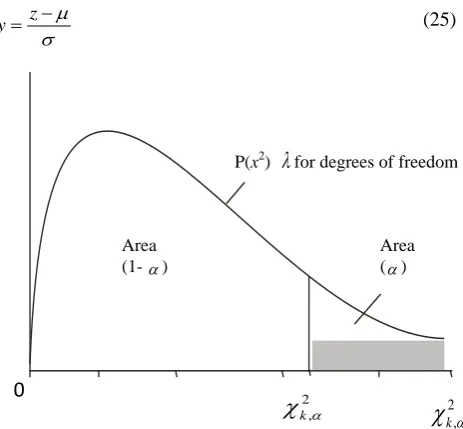
If the measured values are plotted as a function of their relative frequency of occurrence, a histogram is obtained to which a continues curve can be fitted as the number of measurement increases theoretically to any number. The continuous curve commonly encountered is a ball-shaped function p(z). This is the Gaussian or normal probability density function gives as:

 

2 2

1

2 5

1

      

 

  



z z

[image:4.595.301.564.63.322.2]

p (23)

Figure 1: Gaussian normal distribution

The probability that z-takes on values between the point a and b in figure 1 is the shaded area given as;





 

   

 2

1 2

1 ₂1_

 

 





b 

a b

ap zdz b

z a

pr (24)

The total area under the curve p(z) between 0 and equals to 1. The value of z is certain with probability equal to 1 or 100%.

The Gaussian distribution plays a very important role in the measurement statistic because the probability function density cannot be directly integrated. For transfer from z to y using change of variable formula as:

 

  z

y (25)

Figure 2: Gaussian distribution skewed to the right

p(z) p(y)

2

2 1

2 1 )

( 

       

  

p k z

p

Shade area = Pr(c < z <b) = Pr (y < y < yk₎



4 2   b  4

z-scale

y-scale

-4 -2 ₀ y1_yo ₂ ₄

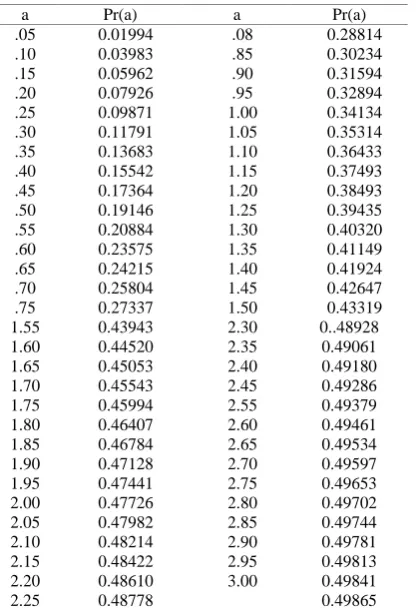
Area (1- )

Area ()

0 ₂

,



_k 2

,



_k [image:4.595.309.541.509.723.2]

(5)

[image:5.595.43.265.75.285.2]

Table I: Normal chi-square distribution table (Values of area

 to the right of 2 , 2



 k  k

k 0.05 0.025 0.01 0.005

1 3.84 5.02 6.64 7.88

2 3.99 7.38 9.21 10.60

3 7.82 9.35 11.35 12.84

4 9.49 11.14 13.28 14.86

5 11.07 12.83 15.09 16.75

6 12.59 14.45 16.81 18.55

7 14.07 16.01 18.48 20.28

8 15.51 17.54 20.09 21.96

9 16.92 19.02 21.67 23.59

10 18.31 20.48 23.21 25.19

11 19.68 21.92 24.73 26.76

12 21.03 23.34 26.22 28.30

13 22.36 24.74 27.69 29.82

14 23.69 26.12 29.14 31.32

15 25.00 27.49 30.58 32.80

16 26.30 28.85 32.00 34.27

17 27.59 30.19 33.41 33.72

18 28.87 31.53 34.81 37.16

19 30.14 32.86 36.19 38.58

[image:5.595.309.549.262.411.2]

20 31.41 34.17 37.57 40.00

Table II: Gaussian distribution for chi-square distribution

a Pr(a) a Pr(a)

.05 0.01994 .08 0.28814

.10 0.03983 .85 0.30234

.15 0.05962 .90 0.31594

.20 0.07926 .95 0.32894

.25 0.09871 1.00 0.34134

.30 0.11791 1.05 0.35314

.35 0.13683 1.10 0.36433

.40 0.15542 1.15 0.37493

.45 0.17364 1.20 0.38493

.50 0.19146 1.25 0.39435

.55 0.20884 1.30 0.40320

.60 0.23575 1.35 0.41149

.65 0.24215 1.40 0.41924

.70 0.25804 1.45 0.42647

.75 0.27337 1.50 0.43319

1.55 0.43943 2.30 0..48928

1.60 0.44520 2.35 0.49061

1.65 0.45053 2.40 0.49180

1.70 0.45543 2.45 0.49286

1.75 0.45994 2.55 0.49379

1.80 0.46407 2.60 0.49461

1.85 0.46784 2.65 0.49534

1.90 0.47128 2.70 0.49597

1.95 0.47441 2.75 0.49653

2.00 0.47726 2.80 0.49702

2.05 0.47982 2.85 0.49744

2.10 0.48214 2.90 0.49781

2.15 0.48422 2.95 0.49813

2.20 0.48610 3.00 0.49841

2.25 0.48778 0.49865

Table III: Data collected from geographical location about laboratory confirmed cases

location/geograhical region

clinical suspected census

laboratory confirmed cases

positive predictive accuracy

Buguma city/south 161 28 17%

Ido town/ south 223 64 30%

Abalama/ south East 181 26 15%

Elelelema town/south

east 32 6 20%

okpo town/south 13 3 24%

Sama /south east 45 13 30%

Kala-Ekwe town/south 4 2 5%

Efoko/ south 33 1 3%

Tombia town/ south east 8 0 0%

IV. RESULTS AND DISCUSSION

The data collected from different geographical location for patients by a physician on malaria epidemic cases were estimated using the developed modified state estimation model for malaria mortality. The measurement statistics are

, 80 120 5 . 1

: ₁ 

  



_z _ _ _mmHg

z ,

80 120 5 . 1

2 

  

  _ _

mmHg

z ,

80 120 8 . 1

3 _

 



 _ _

mmHg z

   



 _ _

mmHg z

80 120 9 . 1

4

while the estimated measurement the model zˆ:



zˆ1 1.4759



,



zˆ2 1.4759



, wand



zˆ₄ 1.87295



. The state estimates of the body blood pressure were determined as x1, x2:8.5225 and

13

.

235

for the respective patients under study, which indicate low-pulse rate or heart rate that required attension, which is also agree with the validated results of the coded matrix laboratory (matlab results).

[image:5.595.45.254.311.617.2]

Fig. 3: A bar chart showing clinical/laboratory confirmed cases.

Fig. 4: A chart showing positive prediction for clinical/laboratory cases

Fig.5: A line chart showing distribution of clinical/laboratory cases.

0 50 100 150 200 250

Co

n

fi

rm

e

d

cl

in

ical

an

d

la

b

or

ar

y

case

s

Geograpghical location of patients

laboratory cnfirmed cases

0% 100%

Co

n

fi

rm

e

d

cl

in

ical

an

d

la

b

or

ar

y

case

s

Geograpghical location of patients

laboratory cnfirmed cases

0 50 100 150 200 250

Co

n

fi

rm

e

d

cl

in

ical

an

d

la

b

or

ar

y

case

s

Geograpghical location of patients

[image:5.595.303.551.437.786.2] [image:5.595.42.288.651.786.2]

(6)

C

Compute the matrix operation: HT_W

Compute for state estimate of the physical measurement

(z) that is:

          

 

   

 

2 1

4 3 2 1

ˆ ˆ x x H

z z z z

Compute the gain matrix (G) operation: HT_WH

Compute the inverse of gain matrix G-1_{operation: H}T_WH

Compute the matrix multiplication operation:

WH H G) T (

Compute the matrix operation:

     



2 1 1

x x WZ H

G T

Where; Z is the physical measurement of the parameter.

C

Calculate the measured parameter (Z) to the percentage (%)

precision of the true or actual value of measurement (xi) into

the modified state estimation model for purpose of accuracy:

4 2 1 4

3 2 1 3

2 2 1 2

1 2 1 1

% 9 % 8

% 8 % 9

% 6 % 8

e x x Z

  

4 2 1

4

3 2 1

3

2 2 1

2

1 2 1

1

009 . 0 08 . 0

08 . 0 09 . 0

06 . 0 8 0 . 0

06 . 0 08 . 0

e x x

Z

e x x

Z

e x x

Z

e x x

Z

 



 



 



 



Formulation of diagonal weighting factor (Wi) of: w1, w2,

w3, w4

Input the state estimation equations characterizing

the physical measurement (Z), true value of the

system model





i ijxj ijxi h e

h   and the addition of

errors term (ei) about the vital statistic variable of

patients for malaria mortality.

Start

Calculate/simulate the modified state estimation algebraic equations as:

Formulation of coefficient matrix (H):

      

22 21

12 11

h h

h h H

   

 

   

 

  



4 3 2 1

W W W W

W

Formulation of coefficient Transpose matrix (H), as

HT_:

      

22 21

12 11

h h

h h HT

(7)

Expected Values of measurements

We assume that the noise terms e₁, e₂, e₃ and e₄, are independent Gaussian random variables with zero means and the respective variances 2

3 2 2 2 1,



,



and



₄2 of the

physical measurement are considered. Two variables are termed independent when

E

 

e

i

e

j



0

fori j. The zero

mean assumption implies that the error in each measurement has equal probability of taking on a positive and negative values of a given magnitudes.

The analysis of the vector (e) and its transpose



e

1

e

2

e

3

e

4



e

T



can be represented as:





    

 

    

 

 

  

 

   

 



2 4 3 4 2 4 1 4

4 3 2 3 2 3 1 3

4 2 3 2 2 2 1 2

4 1 3 1 2 1 2 1

4 3 2 1

e e e e e e e

e e e e

eT (26)

Analysis consideration:

– The expected value of T

ee are found by calculating expected value of each entry in the matrix operations.

– The expected value of all the off diagonal events are zero because errors are assumed to be independent, the expected values of the diagonal events are non zero and correspond to the variance:

 

2

j

e

E

for i from 1 to 4.

– The resultant diagonal matrix are usually assigned the (R) given as:

 



  

 

    



 

 

2 4 2 3 2 2 2 1

. . .

. .

.

. . .

. .

e E e E e E e E

R ee

E T (27)

    

 

    



 



2 4 2 3 2 2 2 1

. . .

. .

.

. . .

. .



(28)

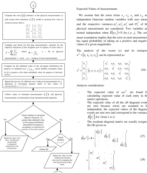
Figure 6: Algorithms (Flow-chart for modified state estimation model for malaria mortality showing different measurement system plan.

Evidently, the statistical properties of the weighted least-square estimation provides solution to the measurement (z), which is the sum of the Gaussian random variables

 

e1 and

the constant term



h

₁₁

x

₁



h

₁₂

x

₂



which represents the true values

z

1_true of

z

1. The addition of the constant term to

shift the curve of

e

₁of the right by the amount of the true value.

Weighting Factor (w)

The analysis of formulating the objective function (f), the preferential weighting

 

w

_i is given to be more accurate measurement by choosing the weight

 

w_i as the reciprocal of the corresponding to the variance



2j. This means that an Output the values of (f)

that is the physical measurement is adequately conducted for true

measurement.

C

Compute the error

 

eˆ estimates of the physical measurements (z)

and system state estimation ₍_zˆ₎ model to measure how close to

system accuracy that is:

   

 

   

 

    

 

   

 

    

 

   

 

4 3 2 1

ˆ ˆ ˆ ˆ

z z z z

e e e e

Repeat the process for different sets of physical measurements by a physician to investigate patients status of true values of

measurements z1, z2, z3, z4

Compute and check for bad data measurements; calculate for the

objective functions (f) the weighted sum of squares of errors that is:





 n

j j

j

e f

1 2 2

 , where 1 j,

W _ n = No of physical

measurement, e = error,  = variance of error measurements.

Compute for the tabulated value of the chi-square distribution for purpose of validation test;



k,

f check whether calculated values

of (f) is greater or less than calculated value for purpose of decision

making.

Collect values of estimated measurements ₍_zˆ₎ and physical

measurements (z) determined, from estimated model equations.

Check whether if calculated

objective function f is

greater than tabulated value of chi-square distribution

determined for purpose f

acceptance or rejection for purpose of decision making.

No Yes

Yes whether:Check

2 ,

k

f 

Output the

value of f

Output the value of f and continue the iteration processes by engaging the

next logical loop in that order.

Stop

[image:7.595.45.544.48.636.2]

(8)

errors of smaller variance have greater weight (w), hence we can specify the weighting matrix, (w) as:

      

 

      



 _



 

2 2

3 2 2 2 1

1

1 . .

.

. 1

. .

1 .

. .

1



R

W (29)

The, gain matrix becomes (G) = HTR–1H (30) The weighted sum of square of error as the objective function (f), determination

The critical value of the statistics f can be determined using the tabulated values of



k2, for a quantifiable level of

significance, k: degree of freedom



N

_m



N

_s



. That is the calculated value can be compared to the tabulated value to measure accuracy which is given as:





2k,





 

1





r

f

X

p

(31)

The weighted sum of squares equation of errors with weight

 

w

i choosen equals to the reciprocal of corresponding error _

    

2

j

δ

variance which is given as:























_



  

 





2 3

2 2 1 3 3

2 2

2 2 1 2 2 2

1 2 2 1 1 1 1

2 2

,

, ,



 



x x h z

x x h z x

x h z e f

N

j j

j









2 4

2 2 1 4

4

,



x

h

z



(32)

Where:

h

₁

,

h

₂

,

h

₃ and

h

4 are function that expresses the

measured quantities in terms of the state variable while

3 2 1

,

e

,

e

and

e

₄are Gaussian random variables terms. The true value of

x

1and

x

2 and not known and have to be

estimated from measurement:

z

₁

,

z

₂

,

z

₃and

z

₄ respectively. Chi-square test statistics (f), as a sum of squares of error terms for purpose of validation

The analysis of physical measurement, the chi-square distribution test and validation are required to the check the presence of bad data. Then eliminate any bad data detected and recalculate subsequent resultant state estimation from the determined results.

The objective function (f) for chi-square distribution can be presented as:

2 4 4 2 3 3 2 2 2 1

2 1 1 2 2

ˆ

e

w

e

w

e

w

e

w

e

f

N

j j

j













(33)

where;

w



1



2

: variance of measurement error

: quantifiable level of significance for accuracy

2 ,K

X

f



_ : for a quantifiable level of significant

 

 for a given degree of freedom (k). If f is greater than X2_,_K then there is at least suspected bad data measurements in the analysis which required attension.

This means that the suspected measurement instrument (z) must be recalculated and subjected to test statistics and required re-measurement of the vital statistics variables of the system.

This could be traceable to human error, instrument error due to poor calibration, aging of the instrument and temperature/humidity etc.

If

f



X

_2_,_Kis satisfied it is adequate for purpose of physical measurement accuracy, while comparing calculated and tabulated values for validation.

Standardized error estimates

The standardized error estimations can be determined using diagonal elements as:

1

Sde

' 11 1

ˆ



R e

2

Sde

' 22 2

ˆ



R

e

(34)

3

Sde

' 33 3

ˆ



R

e

4

Sde

' 44 4

ˆ



R

e

Analysis of measurement for malaria mortality Using modified state estimation model

(9)

measurement carried out by the physician? Which can be represented as:

i

ij

h

Z









(35) Z : Measurement of the vital statistics variable of the patients.

:

ij

h

Account for the precision of the measurements to the accuracy of the instruments (how close to the true value).

i

x : Unknown state variable that need to be determined and accounts for the pulse/health rate for blood pressure measurement.

i



: Error term introduced in the measurement which can be expressed mathematically as:

1 2 12 1 11 h

Z x  h x e (36)

Equation (36), provided the vital statistics variable measurement which is the weighted sum of squared of errors for the Gaussian distribution. Since the physical measurements of the patients is considered as a function of their relative frequency of occurrence, a histogram may be represented which is a continuous curve in relation to the number of occurrence.

Clinical Diagnosis Measurement, geographical location and distribution.

[image:9.595.310.562.87.299.2]

Data were collected from reputable hospitals and clinics from different location for malaria mortality using blood pressure measurements as one of the key associated parameter for the incidence of malaria parasite transmission variable.

Table IV: Distribution of suspected and confirmed cases of malaria parasites (Plasmodium) according to the province in a Developing countries.

S/N

Location/Geogra-phic region

Clinical suspected census (%)

Laboratory confirmed

Positive predictive

accuracy 1. Buguma city/South 161(23) 281 (0) 17% (10 – 24)

2. Ido town/South 223(32) 64(45) 30% (24 – 35)

3. Abalama/South East

181(26) 26(18) 15% (10 – 20)

4. Elelema town/south- cast

32(5) 6(4) 20% (8 – 36)

5. Okpo town/south 13(2) 3(2) 24%(6 – 54)

6. Same south-east 45(6) 13(9) 30%(16 – 44)

7. Kala Ekwe town/south

4(0.6) 2(1) 5%(7 – 93)

8. Efoko/South 33(5) 1(0.7) 3%(0.1 – 16)

9. Tombia/South 8(1) 0 0%(0 – 37)

Total 700 143

Table V: Blood Pressure Measurement (Sphygmomano-meter) for purpose of incidence of malaria parasite transmission

S/N Vital statistics variables for measuring

transmitted cases of malaria parasite (plasmodium) etc

Blood (BP) Pressure Measurement

Accepted standard for blood pressure measurement .

1. Measurement 1; patients - A: Abuja City in Nigeria

5 . 1 80

120



mmHg Ok (normal)

2. Measurement 2; patients –B Buguma City in Nigeria

5 . 1 80

120



mmHg Ok (normal)

3. Measurement 3; Patients –C Lagos City in Nigeria

8 . 1 80

140 _

mmHg Required

attension

4. Measurement 4: Patients – D Port Harcourt City in Nigeria

9 . 1 80

150 _

mmHg Required

attension

Table VI: Sphygmomanometer measurement and precision for true (actual value of measurement) for associated malaria parasite transmission

S/N Measurements instrument Sphygmomanometer (BP)

Precision to the accuracy of measurements instruments 1. Measurements 1, Blood

pressures for pulse rate estimation –Abuja City in Nigeria

8% & 6% to the true values of the system model measured

2. Measurement 2, blood pressure for pulse rate estimation –Buguma City in Nigeria

8% & 6% to the true values of the systems model measured

3. Measurements 3, blood pressure for pulse rate, estimation –Lagos city in Nigeria

9% & 6% to the true values of the systems model measured

4. Measurement 4, blood pressure for pulse rate estimation –Port Harcourt City in Nigeria.

8% & 9% to the true values of the system model measured

Measurements Matrix, (Z) equation given as:

 

        

 

        

 

   

    

 

   

 



9 . 1 80

150

8 . 1 80

140

5 . 1 80

120

5 . 1 80

120

4 3 2 1

mmHg mmHg mmHg mmHg

Z Z Z Z Z

[image:9.595.311.562.348.575.2] [image:9.595.42.282.491.670.2]

(10)

Measurements error (e) given as:

 

To

be

determined

4 3 2 1               e e e e

e (38)

True value of system model term given as:

1

2

12

h

1

11

h

ij

h

x

_



x



x



e



 ₍₃₉₎

Measurement instruments precisions to the accuracy of true/actual value give as:

4 2 % 9 1 % 8 4 3 2 % 8 1 % 8 3 2 2 % 6 1 % 8 2 1 2 % 6 1 % 8 1 e x x Z e x x Z e x x Z e x x Z             (40)

Equation (40) can be represented as:

4

2

09

.

0

1

08

.

0

4

3

2

08

.

0

1

08

.

0

3

2

06

.

0

1

08

.

0

2

1

2

06

.

0

1

08

.

0

1

e

Z

e

Z

e

Z

e

Z









































(41)

Where; x₁ and x2 are the state variable that is unknown that needed to be determined

Case 1: Formulations of the Coefficient matrix (H) which can be represented as:















09

.

0

08

.

0

08

.

0

09

.

0

06

.

0

08

.

0

06

.

0

08

.

0

H

(42)

Case 2: Weighting factor for measuring instrument

 

w

_i which can be presented in diagonal matrix form as:















50

.

50

.

100

.

100

i

w

(43)

Where

w

i



w

1

,

w

2

,

w

3

,

w

4

The weighing factor (w) for the measurement instrument

w

1

,

w

2

,

w

3

,

w

4 are, 100, 100, 50, 50

Case 3: Determine nation of transpose of coefficient matrix (H) given as:

       09 . 0 08 . 0 06 . 0 06 . 0 08 . 0 09 . 0 08 . 0 08 . 0 T H (44)

Case 4: Compute the matrix operation HTW as:



























50

.

50

.

100

.

100

09

.

0

08

.

0

06

.

0

06

.

0

08

.

0

09

.

0

08

.

0

08

.

0

W

H

T (45)















5

.

4

6

4

5

.

4

8

(46) Case 5: Determination of gain matrix (G) given as:

,

Thus

WH

H

G



T

                   09 . 0 08 . 0 08 . 0 09 . 0 06 . 0 08 . 0 06 . 0 08 . 0 5 . 4 4 6 6 4 5 . 4 8 8 G (47) This implies;















445

.

1

68

.

1

68

.

1

005

.

2

WH

H

G

T (48)

Case 6: Determination of Inverse of gain matrix (G) given as:          445 . 1 68 . 1 68 . 1 005 . 2 1 G I

G (49)

074825

.

0



G



















005

.

2

68

.

1

68

.

1

445

.

1

074825

.

0

1

G

(50)

or           9 . 26 45 . 22 45 . 22 3 . 19 1 G (51)

Case 7: Determination of multiplication of inverse operation of gain matrix

 

G1 and HTW given as:

                5 . 4 4 6 6 5 . 4 8 8 8 . 26 45 . 22 45 . 22 3 . 19

1 _H _W

G T

(11)

This implies             8 . 30 175 . 6 8 . 18 8 . 18 825 . 23 95 . 2 7 . 19 7 . 19

1 _H _W

G T

(53)

Case 8: Determination of matrix operation



G1 HTWZ



given as:                         9 . 1 8 . 1 5 . 1 5 . 1 8 . 30 175 . 6 8 . 18 8 . 18 825 . 23 95 . 2 7 . 19 7 . 19 1 WZ H G T (54)

Where; G1 HTWZ is represented as the matrix operations determination of the state variables estimate

x

ˆ

1

and xˆ₂ given as:

               13.235 8.5225 WZ T H 1 G ˆ ˆ 2 1 x x (55) Case 9: Determination of the matrix operation Hx as a function of the estimate of the physical measurements

      4 Z 3 Z 2 Z 1

Z given as:

Xˆ

H

ˆ



Z

(56)



























2

1

ˆ

;

4 3 2 1

X

H

Z

Similarly

(57) Where;                              235 . 13 5225 . 8 2 X 1 X ˆ , 09 . 0 08 . 0 08 . 0 09 . 0 06 . 0 08 . 0 06 . 0 08 . 0 x H (58)

Thus; the estimates of the measurement

 

Zˆ becomes as:

                                     235 . 13 5225 . 8 09 . 0 08 . 0 08 . 0 09 . 0 06 . 0 08 . 0 06 . 0 08 . 0 4 ˆ 3 ˆ 2 ˆ 1 ˆ Z Z Z Z (59)

This implies as:



























87295

.

1

825825

.

1

4759

.

1

4759

.

1

4

ˆ

3

ˆ

2

ˆ

1

ˆ

Z

(60)

Case 10: Determination of number of physical measurement (Nm) and states variable

 

N

_s on the view to determine redundancy

 

K for a quantifiable level of significance.

3 2 1,Z , Z

Z

N_m  and Z4  4 (four physical measurements) 2

& 2

1 

 x x

Ns (blood pressure for pulse/heart

rate)

Redundany (K) N_mN_s 422

(61) Case 11: Determination of errors estimates

 

eˆ of the physical measurements and estimated measurements

 

zˆ are presented as:





 



estimated

measuremen

t

Z



Z

t

measuremen

Physical

e

ˆ

)

(

ˆ





(62) That is;









































3 3 2 1 4 3 2 1 4 3 2 1

ˆ

Z

e

(63) Where;                                                         87295 . 1 825825 . 1 4759 . 1 4759 . 1 ˆ ˆ ˆ ˆ ; 80 / 150 9 . 1 80 / 140 8 . 1 80 / 120 5 . 1 80 120 5 . 1 3 3 2 1 4 3 2 1 Z Z Z Z mmHg Z Z Z Z (64) Thus,





























02705

.

0

025525

.

0

0241

.

0

0241

.

0

ˆ

4 3 2 1

e

(65)

Case 12: Determination of sum of Squared of Errors (e) Measurement

(12)

deduced that there is suspected error (or bad data in the measurement sets).

Similarly,

If calculated objective function (falculated) is less than

chi-square distribution value, it is concluded or declared a vlations which does not satisfy the measurements criteria for decision making for purpose of diagnosing human body conditions.

IV. RESULTS AND DISCUSSION

Case 13: Estimate of measurements error (e)

The objectives function (f) of the weighted sum of squares of errors can be presented as:

2 ) ( 50 2 ) 3 ( 50

2 1

) 2 ( 100 2 ) 1 ( 100 2

2

4

e e

n j

e e

j j e f



 

  





02705 . 0 4 , 025525 . 0 3

, 0241 . 0 2 , 0241 . 0 1 :

 



 

e e

Where

 



 



 



2 ) 02705 . 0 ( 50 2 ) 025525 . 0 ( 50

2 ) 0241 . 0 ( 100 2 ) 0241 . 0 ( 4

1 2 100

2 j

j j e f



) 0007317025 .

0 ( 50 ) 25 0006515256 .

0 ( 50

) 00058081 .

0 ( 100 ) 00058081 .

0 ( 100



 

036585125

.

0

5

0325762812

.

0

058081

.

0

058081

.

0





185323125 .

0



Similarly,

The chi-square distribution from tabulated results given as: 

  



 2 _₉_.₂₁ ,



k

2 ,





k calculated

f 

where;

2

4









s

N

m

N

K

For,





1% quantifiable level of significant = 0.01

) 01 . 0

(

(significance level,



0.01)

The probability of



(1)



10.01



=99% declared confidence level for a degree of freedom,

2







N

s

m

N

K

From the tabulated result obtained for a given degree of freedom and a quantifiable level of significance of

01 . 0



 , for k  2 given as 9.21 which means that the calculated value of

(

f

_calculated

)

is greater than the critical value of the square distribution value. Thus, the chi-square of f provides a test statistics for validating the error measurements of bad data or probably suspected adverse health condition that required attensions for purpose of ensuring good status healthy conditions.

%MATTIX LABORATORY

%PROGRAM :MATLAB FOR MALARIA MORTALITY %AUTHUR : BRAIDE, SEPIRIBO LUCKY

%TECHNICAL PAPER PORESENTAION

%First iteration calculation using a flat start values (,k,t which

%represent the static variables x1 and x2);

k=1; t=1;

% measurement instrument represented as z: z1 z2 z3 z4

z1= 1.5; z2 =1.5; z3 =1.8; z4 =1.9;

z=[1.5; 1.5; 1.8; 1.9];

% estimated measurement represented as zk1 zk2 zk3 zk4

zk1 = 1.4759; zk2 = 1.4759; zk3 = 1.825825; zk4 = 1.87295;

% measurement error represented as e1 e2 e3 e4

e1 = z1-zk1; e2 = z2-zk2; e3 = z3-zk3; e4 = z4-zk4;

% Jacobianmatrix represented as H H = [0.08 0.06;0.08 0.06;0.09 0.08;0.08 0.09];

%Transpose of jacobian matrix T represented as H

T =H'

% Diagonal matrix of the weighting factor as W

W=[100,0,0,0;

0,100,0,0;0,0,50,0;0,0,0,50];

% MUutiply Transpose of jacobian matrix H' and weighting factor W as

D=H'*W

% Mutiply the matrix operation D and jacobian matrix H to obtain gain matrix represented as

G=D*H

% The inverse of gain matrix G represented as F

F=inv(G)

% multiply the matrix operation F and matrix D be represented as

(13)

% multiply matrix M and Z representation as N= M*Z state variable [xi x2]

% Determination of matrix operation of state estimation [x1 x2]=N

for z=[1.5; 1.5; 1.8; 1.9]; v=M*z

end

T =

0.0800 0.0800 0.0900 0.0800 0.0600 0.0600 0.0800 0.0900

D =

8.0000 8.0000 4.5000 4.0000 6.0000 6.0000 4.0000 4.5000

G =

2.0050 1.6800 1.6800 1.4450 F =

19.3117 -22.4524 -22.4524 26.7959 M =

19.7795 19.7795 -2.9068 -23.7888 -18.8440 -18.8440 6.1477 30.7718 v =

8.9075

13.0003

V. RECOMMENDATION

Considering the fact that health is wealth the relationship between the two is frequently misconstrued. That is there is strong need for healthy living to create wealth for man and society.

Measurement of malaria endemictiy is basically on vector or parasites measurement especially for infected cases on transmission of plasmodium parasite etc which may seriously leads to some vital sign and symptom: Temperature rise beyond normal level, headache, blood pressure become abnormal, blood-sugar concentration level may also be affected medically etc.

Evidently, the mapping of malaria transmission have demonstrated a wider geographical distribution of the parasite (plasmodium, etc). The number of clinical report cases due to malaria infection resulted into early mortality which is becoming an increase on daily basis across the world. Particularly in south America, where P.Vivax is currently the most predominant malaria species. Although control measures and programs have had a significant impact on malaria associated cases. Consequently the centers for disease control and prevention(CDC) Saving lives, protecting people in various states of America have considered regular, rapid and accurate diagnosis of malaria which is an integral part to the appropriate treatment of

affected individuals. It is also requested that the CDC: Health care providers should always obtain a travel history form patients, especially person who traveled in a malaria epidemic area, must be evaluated for check using appropriate tests (for malaria) for purpose of healthy free environment. This technical paper having carried out thorough extensive investigation especially to this robust medically affected case of earthly malaria mortality for man which may also be associated to bad measurement for vital statistics variables about a patients. The detail history of patients measured must be checked for accurate, precision, tolerance, error etc to the true value declared by standard world health organization (like WHO etc). Therefore physical measurements taken by medical practioner from patient must:

(i) Regularly check for instrument calibration measurement for effectiveness before drug prescription/administration.

(ii) Consider and satisfy many associated variables measurement to the particular emergence of incidence of malaria species before placing drugs administration and dispensing to avoid over-does or under-dose problems which may leads to early malaria mortality.

(iii) Considering adequate treatments procedures for malaria cases which may depends on disease severity, species of malaria parasites infections on the view to determine the organism that is resistant to certain anti-malarial drugs in order to provide adequate alternative provisions.

(vi) Check for vaccine effectiveness to affected cases of malaria patients particularly to age, sex, community (habitant or group of people) and other associated multivariable’s parameter like vaccination histories etc to avoid gradual destruction of sensitive organs like liver and kidney etc.

(v) Check for bad data measurement: the status of human body state which may be affected by surrounding circumstances, ageing of measuring instrument, human error, temperature/humidity, sensitivity of measurement etc.

(vi) This work can also be extended to include the estimation of malaria mortality the estimation of malaria mortality and recovery rates of plasmodium falciparium parasitaemic, using the model equations:

The transition rates: h and r can be estimated from transition frequencies:



and



with



 





 





  



1 1

ˆ _In

t h



 





 





  



1 1

ˆ In

t r

(14)

t : time interval for estimation h : incidence rate

r : recovery rate

VI. CONCLUSION

The analysis of modified state estimation model is developed for estimated measurement of malaria mortality in a case of a developing countries. This model help to identify detect and flag measurement error which is classified as bad data measurement; whose result may be received on drug prescription and administration for early malaria mortality rate especially when measurement instruments are not regularly calibrated for efficiency. This technical paper for purpose of analysis and scope considered the associated vital statistic variables like blood-pressure (BP) using sphygmomanometer as a key driver for this analysis. The techniques establishes a mathematical modified state estimation model that characterises the physical measurement of the patient to the acceptable value of (BP=

80

120_{mmHg) in order to satisfy the operating normal}

conditions.

The true value of the system model equations and error term addition are considered for purpose of estimating measurements made by physician instrument. Data were collected from four(4) geographical area in a developing countries for purpose of validation of the modified estimation model. The techniques allow for an algebraic summation operation of measurement for the weighted sum provided the declared standard measurement of blood

pressure of _

  

 

ed not violat is 80 120

Hg mm

The analysis technical paper identified bad data measurement which required urgent attention for check: The surrounding circumstance of the patients, human error, calibration error etc for the purpose of determining the state of the body system configuration.

The paper also validated this work research via the objective function (f) as the calculated value versus chi-square distribution (tabular form) for 99% level of significance with 2 degree of freedom in quantitative measures.

This paper also establishes a string conformity, uniquencie and synergy between measured ad estimated measurements which eventually validated with objective function calculated (f) and chi-square distribution and between matrix operations and matrix laboratory code programs for a test statistics.

REFERENCES

[1] Guerra CA, Snow RW, Hay SI (2006) Mapping the global extent of malaria In 2005. Trends Parasltology 22:353-358.

[2] Guerra CA, Howes RE, Patll AP, Gething PW, Van Boeckel TP, et al. (2010) The International limits and population at risk of Plasmadi transmission in 2009. PLoS Neglected Tropical Diseases 4:e774. [3] Price RN, Tjitra E, Gunrra CA, Young S, Whlto

NJ, at al, (2007) Vivax malaria; neglected and not benign, The American Journal of Trc