Abstract— This paper presents a novelty model for solving a routing problem for delivery service using EV trucks called electric vehicle routing problem (EVRP). We also present a meta-heuristic algorithm by combining genetic algorithm and Tabu Search algorithm, to solve the EVRP. The difficulty of using a EV truck for a good delivery service is finding out an optimal route in a huge number of rotes. additionally, it also need to consider the short driving distance problem because of battery limited of EV. The formulation present was based on a mixed integer programming formulation, objective to minimum the total electrical consumption and multiple constraints, which considered the electric recovery in a gradient road and arrange the loading assignment, to improve the electrical consumption efficiency. additionally, the electrical consumption balance of every trucks was considered. It good to reduce the charging operation time and improve the operations efficiency for this problem.
We designed and executed five experiments to evaluate our formulation and algorithm, verified the effectiveness of our idea in EVRP problem. Experiments show that, the total electrical consumption calculated by proposed EVRP model could be improved 2.3% than a conventional VRP model, and the operations time balance objective made 48.3%’s reducing of charging operation time.
Index electric vehicle routing problem, optimization, genetic algorithm
I. INTRODUCTION
RUCKS were used for more than 90% ′s freight transportation in Japan[1]. The large numbers of trucks, made emissions caused air pollution. it was also affected by the oil crisis. Nowadays, there was a demand for replacing traditional diesel vehicles with clean energy vehicles. how to find an optimal route, which could let EV truck deliver all customers with a minimum cost. Additional, if we want to help the delivery companies to use EV truck for delivery service actively, we need to face another problem of short travel distance.
In this problem, how to make a route plan, which could let the EV trucks reduce distance, loading weigh was a problem. because of huge numbers of routes combines, if the customer numbers grow up, the routes combine will have a series of
Manuscript received December 20, 2018; revised January 27, 2019. Mr. Hong Chen. Master student of Graduate School of Information, Production and Systems, Waseda University, Kitakyushu-city, Fukuoka 808-0315. ([email protected])
Prof. Tomohiro Murata, Professor of Graduate School of Information, Production and Systems, Waseda University, Kitakyushu-city, Fukuoka 808-0315. ([email protected])
growth. The Different routes combines will have a different result, it’s hard to find out an optimal solving in this. This kind of problem was called NP-Hard problem. Additional for this, because of using EV truck, we also need to search the good features of EV, to improve the delivery ability, that’s electric recovery system, it’s effective when EV truck are travelling on descending road, so the gradient road was also needed to be considered in this problem, and it became more difficulty because of there were more routs combines with considering gradient road.
Conventional researches related to VRP, it’s almost focus on minimum travel distance of fuel vehicle. There were also some various of VRP, like CVRP, VRPTW, MDVRP, Green-VRP etc. [2]. It’s very fewer research related to EV truck’s problem. We defined the electric vehicle truck routing problem(EVRP), We purpose to create a novel method, which could make an optimal routing for letting EV trucks has the minimum electrical consumption, with considering full use the EV trucks electrical recovery system, let our method fit the bottleneck of electric capacity of EV.
Fig.1. Global electric-vehicle sales, 2010-2017. [3]
II. PROBLEM DESCRIPTION
A. Electric Vehicle Routing Problem
We define an Electric Vehicle Routing Problem (EVRP) in this research, it’s objective to
1. Minimum the electric consumption for delivery services by considering energy recovery function of EV truck.
2. Battery charging time balance.
With a novel energy consumption model of EV by considering speed mode, road gradient and load assignment.
Optimal Electric Vehicle Routing for
Minimizing Electrical Energy Consumption
Based on Hybrid Genetic Algorithm
Hong Chen, Tomohiro Murata
B. Electric consumption model
[image:2.595.84.246.117.193.2]There are four kinds of resistance on a traveling truck, air resistance, rolling resistance, gradient resistance, and accelerate resistance.
Fig.2. Resistance of a running truck.
The product of the resistance and distance is the energy consumption of the EV truck.
2
( / 2 sin ) *
EC SV mgmg ma D
ρ: air density
m: weight of vehicle and cargo λ: air resistance coefficient S: projected area of front of vehicle
V: Speed of vehicle Speed mode effect to electric consumption
μ: rolling resistance coefficient g: gravitational acceleration θ: slope degree of road a: acceleration
D: travel distance
1) Load assignment effect to electric consumption
[image:2.595.97.231.549.649.2]The mass of cargo affects to rolling resistance, gradient resistance, and accelerate resistance, it means affect to the electric consumption. Making an optimal load dispatching plan, will help truck to reduce the energy consumption.
Fig. 3. Calculation method of gradient resistance.
C. Electric recovery model
For an EV truck, it could recover the electric energy when it is descending a hill.
2
( sin ( / 2 )) *
EO mg SV mg D
III. FORMULATION AND SOLVE APPROACH
A. Formulation of problem
G.B. Dantzing and J.H.Ramser proposed an optimal formulation for a vehicle routing problem (VRP) in 1959, it objective to make traveled distance minimum[4].Teruji Sekozawa et al, propose a formulation, objective to maximum the customer number service by one EV truck[5]. In this research, we propose an optimization problem formulation, which objective as minimum the electric energy consumption for this EVRP.
<Notation>
N: number of customers.
K: number of vehicles. (Decision variable)
Cij: the electric consumption between node i and node j.
ECij: electric consumption from node i to node j.
EOij: recovery electric from node i to node j.
Aik: the load level of vehicle k when leaving from node i.
xijk: the binary variable of vehicle k, to run in road between node i and node j. (Decision variable)
B: the capacity of vehicle battery.
W: the load capacity of one vehicle.
ai: the demand of node i.
yik: the binary variable of vehicle k assignment to node I or not.
the formulation of the EVRP is as follow, Objective
1 0 1
min ( , ) min
K V V
k
ijk ij i ijk
k i j
E K X C A X
(1)Subject to
0
1,... 0,...,
i N k k ij i i jk i
C A x R B k K j N
(2)0
1 1,... 0,...,
ijk N
i
x k K j N
(3)0
1 1,... 0,...,
ijk N
j
x k K i N
(4)0
0 1 1,...
k k N i i j
A x k K
(5)1,... 0,...,
k k
j i j ijk
A A a x k K j N (6)
0
1 1,...
N
i ik
i
a y k K
(7)0
1,... 0,...,
ijk i
N
k i
x y k K j N
(8)0
1,... 0,...,
ijk i
N
k j
x y k K i N
(9)0
, 0 1, 1,...,
i K k k K i y i n
(10)2
0
( i 0.8 ) 0.04 1,..., 0,...,
N
i j
C B B i N j N
(11)0,
0,..., 0,..., 1,... 1
ijk
x i N j N k K
(12)
ij i ij
The formulation is a mixed integer programming, calculate the product of electric consumption (Cij), load level (Aij) and routing option of each truck (Xijk). (2) is ensure the traveling truck limited in battery capacity. (3), (4) keep each customer destinations were visited once only. (5) ~ (10) were load constraint, make sure the cargo weight limited in truck loading capacity and find out an optimal load assignment for minimum electric consumption as well. (11) is a constraint for keeping each truck has a similar electric consumption, to balance the working time of drivers.
2
1 0 1
min ( ( , ))
K N N
k
ij i ijk ijk
k i j
C A X E K X
(16) [image:3.595.319.546.234.464.2]
We add an additional objective for this formulation, purpose to keep balance of every trucks’ operations time. We consider the truck need to be charging when they back depot or charging station. The time of this charging operation is MAX (t(v1), t(v2), t(vk)) (t(vk) is the charging operation time of vehicle k), the max time of charging time of a vehicle decided the charging operation time. If we reduce the max charging operations time of a vehicle, it’s good to improve the economics of EV application in business. (16) could let the all of vehicles have the similar electric consumption in work. It means the charging time will be the similar because of the battery size is same as well.
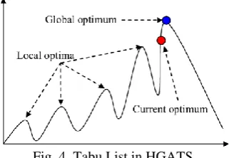
Fig. 4. Tabu List in HGATS.
B. Solving algorithm
EVRP is a kind of combinatorial optimization problem, as a NP-hard problem, in this research we consider choosing Genetic algorithm and Tabu Search of two kind of meta-heuristic to solve it.
In this research, we combine the GA and Tabu Search (TS). Apply the TS as a local search help GA improve the local searchability, control prematurity and to avoid converging to local optimum. Let GA provide a better feasible solution for TS as the initial solution, considering this will help TS reduce the searching time and improve the quality of the result.
Fig. 5. Encoding and duplicate check in GA.
1) Genetic algorithm(GA)
Base on GA, a very popular heuristic algorithm to solve a combination problem. the advantage of GA was simple to do a coding for a VRP problem, and more suitable to solve a large size problem than a Mathematical programming method.
2) Tabu Search(TS)
To help pure GA, climb up local search to find the optimal solution, we combined Tabu search into GA, used a Tabu List to store the feasible solution, to avoid it was a local optimal solution. Tabu Search as a kind of local search, search the optimal solution in the neighborhood, and avoid the local optimal solution with a Tabu list.
Generate solution x Generate N*(x)
Evaluate x’ solution Choose the best x’ in N* and set x=x’
Update Tabu list and best solution
fond so far
N
Y
Generate initial solution
Evaluate population
Output results Selection Crossover Mutation
Gen>Max Ge
Stop conditions Fitness function
Gen=Gen+1
Y N
0 1 2 10 25 0
[image:3.595.93.254.390.501.2]GA TS
Fig. 6. Flowchart of HGATS.
IV. EXPERIMENTS
Prepared two experiments to evaluate the solution’s optimal calculated with HGATS algorithm and the effeteness of proposed EVRP model.
A. Common condition and data for the experiment
Base on the Wakamatsu-ku, Kitakyusyu-city, Japan area(71.31km2), some destination will be take randomly in this area in experiment1 and experiment2.
1) Area,
Base on the Wakamatsu-ku, Kitakyusyu-city, Fukuoka, Japan area(71.31km2), some destination will be take randomly in this area in experiment1 and experiment2.
2) EV,
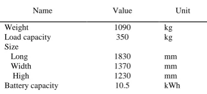
We choose the Minicab of Mitsubishi Motors Japan, as a source EV in these 2 experiments. The main measures of the vehicle were written in tableⅠ.
B. The evaluation of electric saving with EVRP model
[image:3.595.62.267.679.745.2]distance respectively of we proposed EVRP model and conventional VRP model.
Fig. 7. The map of Wakamatsu-Ku, Kitakyusyu-city, Fukuoka, Japan area.
TABLEI PARAMETERS OF EV-MINICAB
Name Value Unit Weight 1090 kg Load capacity 350 kg Size
Long 1830 mm Width 1370 mm High 1230 mm Battery capacity 10.5 kWh
[image:4.595.306.550.113.245.2]Fig 8 shows the electrical consumption difference calculated by EVRP model and conventional VRP model. proposed EVRP has less electrical consumption than conventional VRP model. the EVRP model helps electrical saving in these cases. the electrical saving rates from 0.469%~6.598%. the saving rates is growing up with gradient road rates. We consider that the electrical recovery systems help trucks recovery more electric in higher gradient road rates.
Fig. 8. Electrical consumption comparison between EVRP and VRP.
Fig 9 shows the distance difference calculated by EVRP model and conventional VRP model. The results of VRP model had less distance than the EVRP’s.
Fig 10 and Fig 11 shows the routes result calculated by EVRP and VRP. The different routes in yellow area. Because
node 7 is higher than node 6 and node6 is higher than node 1, we consider that the route of 7 to 6 and route of 6 to 1 both help to recovery the electric in EVRP, but VRP model could not find those routes.
[image:4.595.303.549.294.568.2]Fig. 9. Distance comparison between EVRP and VRP.
Fig. 10. The routes calculated by EVRP model.
Fig. 11. The routes calculated by conventional VRP model.
C. Optimal solution calculated by HGATS’s evaluation
In the second experiment, we want to evaluate the optimal solution calculated by proposed HGATS algorithm.
We calculated the 50% gradient road rates case at last experiment (B) with IBM ILOG Complex solver. In this small size problem, the best solution calculated by proposed HGATS algorithm was the same as calculated by ILOG solver. The results as follows,
[image:4.595.68.270.310.402.2] [image:4.595.47.292.547.684.2]Numbers of vehicle: 2 The route details of 2 vehicles,
[image:5.595.47.291.112.253.2]Vehicle 1, depot-> 0->4->8->9->10->7->6->1->depot Vehicle 2, depot->3->5->2->depot
Fig. 12. Distribution of the fitness of HGATS. Fig 12 shows the solutions from HGATS running 100 times, the mean value was 8.944 kWH, higher than best solution (= optimal solution)20.49%.
To evaluate the performance of HGTS, we executed different size problem from 10 nodes to 70 by HGATS and ILOG solver.
Fig 13 shows ILOG solver had taken 4.19 hours to get a solution when a problems size was 30. For HGATS, it just took 28.929 seconds, ILOG calculating time is 521 times of HGATS algorithms. But for a small size problem, less than 15 nodes, ILOG solver has better performance than HGATS algorithms, of course, the ILOG solver could get optimal solutions every time. So, we consider ILOG solver has a good performance for calculating a EVRP problem if the size was less than 20, otherwise the HGATS algorithm is a better performance.
TABLEⅡ DEMAND OF EVERY CUSTOMER
location Demand(kg) 1 200 2 100 3 50 4 50 5 10 6 10 7 200 8 150 9 150 10 150
D. Effectives of EVRP proposed evaluation
In the third experiment, we selected 10 destinations, with 4 vehicles. The demand of 10 destinations shown below,
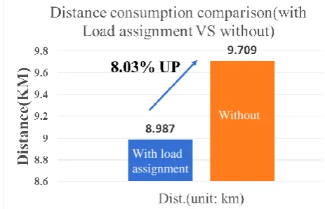
Fig 14 shows the route result with 4 vehicles and 10 customers. Fig 15 shows comparison results of the model with load assignment and not. the left bar shows the result from the model without load assignment consideration, use the average load weight for a vehicle. The right bar shows the results from the model with load assignment consideration, to calculate the electric consumption with different demand of 10 locations, limited load capacity for a vehicle. Fig 16 shows the
difference between the EVRP model with load assignment and without load assignment. The load assignment helped EV trucks’ total electrical consumption reduce 8.84%. it’s also increased 8.03%’s distance. The EVRP model will be useful if the delivery company prefers to low electrical consumption.
0 1000 2000 3000 4000 5000 6000 7000 8000 9000 10000
0 10 20 30 40 50 60 70
T
im
e
(s
e
c
ond
)
Problem Size
Computing time (ILOG VS HGATS)
0 10 20 30 40 50 60
0 10 20 30
T
im
e
(s
e
c
ond)
Problem Size ILOG VS HGATS(Size:0~30)
1 hour
0.5 hour
ILOG
HGATS ILOG
[image:5.595.314.550.322.509.2]HGATS
Fig. 13. Computing time comparison between ILOG and HGATS.
Fig. 14. Solution of the model with load assignment consideration.
Fig. 15. The difference of electrical consumption between within load assignment and without.
E. Evaluate additional objective of operation time balance
In the fourth experiment, we evaluated the operation time balance objective additionally, with a two-trucks and 10-customers’ case.
With load assignment
[image:5.595.315.546.463.674.2] [image:5.595.113.223.516.636.2]We considered the charging operations for multiple truck. Assume that, there were enough charging sets in a charging station. The operation time of charging, will determined by the longest charging time of a truck.
Fig. 16. The difference of distance between within load assignment and without.
[image:6.595.58.292.393.562.2] [image:6.595.56.293.394.749.2]Fig 17 shows the mean value of total electrical consumption from 4.2 kWH to 4.6 kWH, but we could find that the total operation time (*) will reduce 48.3% shown in Fig 18. The operation time calculated based charging set (7 hours/AC200V/15A) from on Mitsubishi Motor cars, assumption of [6]
Fig. 17. Electrical consumption of EVRP model with operation time balance and without.
Fig. 18. Operation time of EVRP model with operation time balance and without.
V. CONCLUSION
(1) Proposed a novel optimization model for EVRP, which improved the EV Truck's efficiency with considering recovery electric and rationalize the load to reduce the electric consumption. It's verified effective to solve the EVRP. (2) Proposed algorithm for solving the EVRP was effective. The solutions were close to an optimal solution. especially, it's fit to a real-world problem, with a big size.
(3) Designed and executed four experiments, to evaluate the model proposed.
ACKNOWLEDGMENT
In this research, I want to thank my professor Murata Tomohiro, who gave a lot very useful and creatable advises to help me in research, let me could be find the problem clearly, to formulate the problem, create an approach to solve it and do an experiment for evaluating it. This a hard process
REFERENCES
[1] 次世代自動車普及戦略[Vehicle diffusion strategy in next generation ],Ministry of the Environment Government of Japan,
http://www.env.go.jp/air/report/h21-01/index.html
[2] Canhong Lin, K.L. Choy, T.T.S Ho, S.H. Chung, H.Y.Lam, Survey of Green Vehicle Routing Problem: Past and future trends,Expert Systems with Applications Vol.41,pp.1118-1138,014.
[3] EV-Volumes.com HP, McKinsey, analysis,
https://www.mckinsey.com/industries/automotive-and-assembly/our-insights/the-global-electric-vehicle-market-is-amped-up-and-on-the-rise.
[4] B.Dantzing, J.H.Ramser (Oct., 1959),The Truck Dispatching Problem, Management Science, Vol.6, No.1, pp.80-91
[5] Teruji Sekozawa, Susumu Yamamoto, Kazuaki Masuda (2014), Maximization of EV Tour Points: The Problem and a Solution, Journal of IEEJ Transactions on Electronics, Information and Systems, Vol.134 No.6 pp.773-779
[6] MITSUBISHI MOTORS home page,
https://www.mitsubishi-motors.co.jp/lineup/i-miev/usp/charging.html
Without With load
assignment
Without
operation time balance
With
operation time balance
With load assignment
Without
operation time
balance Withoperation
[image:6.595.56.293.589.753.2]