CFD modelling of the cross flow through normal triangular tube arrays with one tube undergoing forced vibrations or fluidelastic instability

School of Engineering

Department of Mechanical & Manufacturing Engineering

CFD modelling of the cross-flow

through normal triangular tube arrays

with one tube undergoing forced

vibrations or fluidelastic instability

Beatriz de Pedro, Jorge Parrondo, Craig Meskell, Jesús Fernández Oro

Published in Journal of Fluids and Structures (2016)

CITATION INFORMATION:

“CFD modelling of the cross-flow through normal triangular tube arrays with one tube undergoing forced vibrations or fluidelastic instability” B de Pedro, J. Parrondo, C. Meskell, J.F. Oro, Journal of Fluids and Structures, Volume 64, (2016), Pages 67–86

CFD modelling of the cross-flow through normal

triangular tube arrays with one tube undergoing forced

vibrations or fluidelastic instability.

Beatriz de Pedroa∗, Jorge Parrondoa, Craig Meskellb, Jes´us Fern´andez Oroa

a_{School of Engineering, Univeristy of Oviedo, Spain} b_{Trinity College Dublin, Ireland}

Abstract

A CFD methodology involving structure motion and dynamic re-meshing

has been optimized and applied to simulate the unsteady flow through

nor-mal triangular cylinder arrays with one single tube undergoing either forced

oscillations or self-excited oscillations due to damping-controlled fluidelastic

instability. The procedure is based on 2D URANS computations with a

com-mercial CFD code, complemented with user defined functions to incorporate

the motion of the vibrating tube. The simulation procedure was applied to

several configurations with experimental data available in the literature in

order to contrast predictions at different calculation levels. This included

static conditions (pressure distribution), forced vibrations (lift delay relative

to tube motion) and self-excited vibrations (critical velocity for fluidelastic

instability). Besides, the simulation methodology was used to analyze the

propagation of perturbations along the cross-flow and, finally, to explore the

effect on the critical velocity of the Reynolds number, the pitch-to-diameter

ratio and the degrees of freedom of the vibrating cylinder.

Keywords:

Fluidelastic Instability, Numerical model, Tube arrays, Critical velocity,

Disturbance propagation

1. Introduction

Cylinder arrays subject to cross-flow such as in shell-and-tube heat

ex-changers may undergo self-excited vibrations of high amplitude and high

po-tential for structural damage (Weaver and Fitzpatrick (1988); Pettigrew and

Taylor (2003a); Pettigrew and Taylor (2003b)). The phenomenon, which

is referred to as fluidelastic instability (FEI), can be triggered by either a

fluid-damping controlled mechanism, which only requires motion of one tube

with one degree of freedom, or a fluid-stiffness controlled mechanism, which

requires the coupled motion of several tubes (Chen (1983a); Chen (1983b);

Paidoussis and Price (1988)). FEI has been largely studied experimentally in

the past, with the main purpose of establishing critical flow velocities as the

limiting conditions that ensure stability. However, the data collected of

crit-ical velocity for each main geometrcrit-ical configuration usually show significant

scatter. This is attributed to the wide variety of factors with potential to

influence the phenomenon, including pitch ratio (P/d), number of rows and

columns in the array, degrees of freedom, accuracy of cylinder position in the

array, details of structural parameters of each cylinder in the array, Reynolds

number, turbulence intensity and presence of other excitation mechanisms.

veloc-ity can be obtained by means of the so-called unsteady flow model (Chen

(1983a); Chen (1983b)), but it requires the previous determination (usually

experimentally) of an extensive set of dynamic force coefficients that

rep-resent terms dependent on tube position, velocity and acceleration. These

force coefficients are not easy to obtain and are strongly dependent on

ge-ometry and reduced velocity. Because of that, several theoretical models

have been proposed intended to yield critical conditions for FEI from the

estimation of the fluid forces on the tubes, based on different simplifying

assumptions (Price (1995)). For instance, the so-called quasi-steady model

by Price and Paidoussis (1984) assumes that the fluid-dynamic forces on the

tubes can be obtained by performing static flow calculations with a

cylin-der slightly shifted from equilibrium and then introducing a phase delay for

the resulting static forces. Later, Granger and Paidoussis (1996) proposed a

more elaborated quasi-unsteady model in which the fluid-dynamic forces are

expressed as a combination of transient functions, in order to represent the

memory effect induced in the flow due to the diffusion and convection of thin

vorticity layers from the surface of the vibrating cylinders. Requiring much

less empirical input, Lever and Weaver (1986a), developed a semi-analytical

model in which the flow passes through the arrays along wavy streamtubes

whose cross area fluctuates lagging the motion of the neighboring vibrating

cylinders. In this simplified system, the fluid-dynamic forces on the

cylin-ders can be computed by applying the 1D unsteady flow equations (Lever

and Weaver (1986b)).

phe-nomena up to some extent, but their flow simplifications and the need for

empirical data limit their effectiveness as prediction tools. Indeed, the best

potential for the detailed description of the flow without empirical data

cor-responds to CFD models and that capability should allow for more reliable

predictions of the critical velocity for FEI. Moreover, CFD offers the

possi-bility of simulating the dynamic response of the flow-structure system even

operating at unstable regimes, for which the non-linear terms are dominant.

The latter is key to explore possible new situations involving FEI

phenom-ena, such as in the area of fluid kinetic energy conversion.

In recent years, several researchers have applied CFD models to analyze

the dynamic flow-structure interaction that leads to FEI. Particular attention

has been paid to the case of arrays with only one flexible cylinder undergoing

forced vibrations, because it is convenient to study the correlation between

tube motion and the associated flow fluctuations. Hassan et al. (2010) used

CFD simulations for in-line and normal triangular arrays with one cylinder

subject to forced vibration in order to estimate the unsteady force coefficients

on the tubes. After verifying good agreement between predicted critical

ve-locities and experimental data, they further investigated the effects of pitch

ratio and Reynolds number. This approach was later extended to explore

the delay of the perturbations induced in the flow by an oscillating

cylin-der in a normal triangular array (Hassan and El Bouzidi (2012)) as well as

the corresponding fluctuations in the cross-area of the passing streamtubes

(El Bouzidi and Hassan (2015)). Khalifa et al. (2013b) performed CFD

to model the velocity fluctuations previously measured in wind tunnel

(Khal-ifa et al. (2013a)) and to extend their analysis to lower reduced velocities.

They obtained good correlation between predictions and measurements, and,

besides, they obtained improved estimations of critical velocity when

intro-ducing a CFD derived phase lag function in the model by Lever and Weaver

(1986a), Lever and Weaver (1986b). Following a different approach,

Ander-son et al. (2014) developed a simplified numerical model for a small in-line

group of cylinders, one of them oscillating, with special focus on the

tempo-ral variations induced in the boundary layers and, ovetempo-rall, on the regions of

flow attachment and separation. They concluded that the effective time lag

between fluid forces and tube motion has two components dependent on flow

velocity and vibration amplitude respectively.

In line with these investigations, this paper presents a CFD study on the

fluid-dynamic vibrations due to damping-controlled FEI of one single flexible

tube in normal triangular arrays. The simulations were developed with the

ANSYS-Fluent 12.1 software (ANSYS (2013)). The model incorporates the

motion of vibrating cylinders by means of a special User Defined Function,

so that the domain is remeshed at every time step. First, the main

calcula-tion parameters including boundary condicalcula-tions and turbulence model were

selected by contrasting the predictions of pressure distribution on cylinders

with the measurements conducted by Mahon and Meskell (2009) under static

conditions. Then, dynamic simulations with one oscillating tube located at

the third row were carried out for the sets of configurations tested by Mahon

and Popp (1995) under conditions of self-excited vibration. This

method-ology, which pursued the validation of the CFD model at different levels of

calculation, is depicted in Fig.1. Finally, simulations were conducted to

ex-plore the effects of Reynolds number, pitch ratio and degrees of freedom of

the vibrating cylinder.

2. CFD Model and Static Calculations

For this study, several normal triangular tube arrays were considered with

pitch-to-diameter ratios between 1.25 to 1.58, including the value of 1.32 that

Mahon and Meskell (2009, 2013) used in their experiments as well as the

val-ues of 1.25 and 1.375 used by Austermann and Popp (1995). In all cases, the

array consisted of five rows of six cylinders, as shown in Fig.2. The cylinder

diameter was always 38 mm.

For the simulations involving cylinder motion, the flexible cylinder was

allocated in the third row (tube TV in Fig. 2). According to the

experi-mental study by Austermann and Popp (1995), that position for the flexible

tube would yield the lowest critical velocity for damping-controlled FEI of

normal triangular arrays with P/d=1.25, and also with P/d=1.375 if the

mass-damping parameter is less than about 30.

The calculation domain extended both upstream and downstream from

the cylinder array with lengths equivalent to nine tube diameters.

showed the presence of large scale oscillations in the region downstream the

array. While this type of oscillations may actually take place in practice

(Olinto et al. (2009); de Paula et al. (2012)), they are not considered to be

related to the FEI mechanism. Hassan et al. (2010) also observed this

be-haviour in their computations and they decided to truncate the domain from

the last row of the array as a means to suppress the appearance of those

large scale structures. However, this procedure implies imposing boundary

conditions (constant outlet pressure) on the flow through the array itself, and

that may affect the propagation of disturbances throughout the flow, which is

crucial for the development of the FEI phenomenon. In the present model, as

an alternative strategy to allow for a reasonable distance between array and

domain outlet while preventing large scale oscillations, full-slip guide plates

were placed behind each tube of the last row, parallel to main stream (Fig.2).

To discretize the domain, a specially refined grid was used around each

cylinder in the array that was composed of quadrilateral cells with an initial

thickness of 0.06 mm at the tube wall and a growth factor of 1.15 in the

radial direction until the 13th line. This ensured y+ values of the order of 1

for all the simulations conducted. The rest of the domain was meshed with

triangular cells of progressively greater size when separating from the array.

In order to prepare the model to deal with cylinder oscillations, a

hexag-onal region was defined surrounding the vibrating tube (Fig.2), in which the

triangular cells could either shrink or expand depending on the instantaneous

the oscillating tube moved without undergoing deformation. This approach

meant that, during computations involving cylinder motion, the mesh did

not degrade with excessive distortion for cylinder displacements well above

4% of the tube diameter even for the smallest pitch-to-diameter ratio of 1.25

(as shown in Fig.3).

To begin with, a series of computations was performed under static

con-ditions, i.e. no tube vibration. These tests were intended to select the most

appropriate calculation parameters when comparing predictions to the wind

tunnel data obtained by Mahon and Meskell (2009), who measured the static

pressure distribution around the surface of cylinder labeled TV in Fig.2 for

the caseP/d=1.32 and several cross-flow velocities. These pressure data have

been non-dimensionalized by defining the pressure coefficient:

P∗ = Ps(θ₁)−Ps0

2ρU

2

p

+ 1 (1)

where Ps is the static pressure at location θ on the tube surface, Ps0 is the

maximum static pressure (atθ=0◦),ρis the fluid density and Up is the pitch

velocity. As an example, Fig.4 compares Mahon and Meskell’s experimental

data to the predictions obtained for an upstream air velocity of 2 m/s when

using three different turbulence models: a standard k −ω, a k −ω with

shear stress transport corrections (k−ω SST) and ak−ϵ with

renormaliza-tion group (k−ϵRNG) complemented with non-equilibrium wall treatment

rea-sonably well the experimental data, although the standardk−ω model gives

the closest fit in the wake region. This is within expectations since k −ω

models are considered more appropriate than k−ϵ to deal with separated

flow areas, but in the case of closely packed arrays that feature is less relevant

than in cases of unconstrained wakes.

On the other hand, the two k −ω models are seen to be more prone

to yield asymmetric predictions of pressure around the cylinders than the

k −ϵ RNG. Different degrees of flow asymmetry depending on the

turbu-lence model can be also observed in the computations reported by Iacovides

et al. (2014), who used detailed LES simulations of the flow across an in-line

square array to contrast the predictions from RANS simulations with five

different turbulence models. Interestingly, the predictions closest to the LES

results corresponded to the k −ϵ model in that study. Since the FEI

phe-nomenon is usually associated to vibrations in the transverse direction, it is

key to estimate accurately the lift forces and they are mostly influenced by

the pressure unbalance at the regions around Θ = 90◦ and Θ = 270◦ (Fig.

4), where pressure is minimum. According to this criterion the k−ϵ RNG

model was selected for the subsequent computations.

Another computation series explored the effect of the type of boundary

condition at the channel sides downstream of the array. Specifically, first

they were modeled as full-slip walls and secondly as planes with periodic

repetition of the flow variables. Fig.5 shows the respective pressure

and T8 in Fig.2. Again, some degree of flow asymmetry can be expected

during the iteration process between different cylinders even if they belong

to the same row. The periodic boundary condition is not necessarily

sym-metrical, since strictly it imposes the limitation that the flow field is C1

continuous across the boundary. Despite this, in the present case it was seen

to produce the most symmetrical flow in the domain (Fig.5b), with pressure

distributions around the three cylinders that are almost identical. This can

be attributed to the less rigid restrictions imposed on the flow by the periodic

boundaries (for instance, they allow through-flow), which favor the

attenua-tion of possible symmetrical disturbances formed during the computaattenua-tional

process downstream the half cylinders at the channel sides. In consequence

the boundary conditions at the channel sides were defined as periodic for

the rest of cases tested. This symmetric pattern for the stream can also be

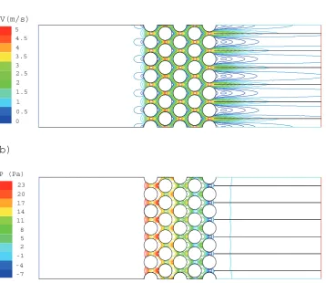
appreciated in Fig.6, which shows typical contours of velocity magnitude and

static pressure obtained from steady flow simulations.

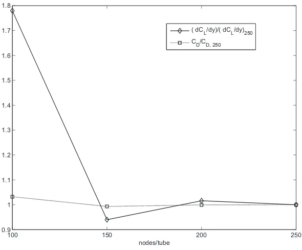
Finally, the effect of cell size was analyzed by comparing the fluid forces

computed for meshes with four different refinement degrees. Each mesh was

characterized by the number of cells adjacent to each tube along its perimeter,

which varied between 100 and 250. In particular the reference magnitudes

considered for contrast were the derivative of the lift coefficient on tube TV

(Fig.2) with respect to its transverse position and the drag coefficient at

neutral position, which are the relevant parameters used in the quasi-steady

theory by Price and Paidoussis (1984). In each case, the derivative of the lift

from calculated lift force data on tube TV when it was held apart from its

neutral position at±0.5% of tube diameter in the transverse direction. Fig.7

shows the results obtained for the array of P/d = 1.25, expressed in values

relative to the data for the most refined mesh. It is seen that above 150 nodes

per tube mesh the differences both in drag and lift derivative are reasonably

small. The bulk of the simulations reported in this paper corresponds to the

mesh with 200 nodes/tube, for which the difference with respect to the 250

nodes/tube mesh was less than 1.6% for the lift derivative and 0.06% for the

drag. The corresponding total number of cells in the domain ranged from

2.8×105 for P/d= 1.25 to 4×105 for P/d=1.58.

3. Forced oscillations in the transverse direction

3.1. Flow fluctuations

The first series of dynamic simulations corresponded to the case of tube

TV in motion under harmonic forced oscillation in the transverse direction,

in order to explore the transmission of perturbations along the air stream

through the array. For that purpose, a special routine (User Defined

Func-tion, ANSYS (2013)) was coupled to the CFD code so that the tube position

and velocity, as well as the domain grid, could be conveniently updated at

every time step during calculations. In addition, fifteen points were selected

along a stream channel that passes by tube TV (Fig.8), in order to monitor

their velocity vector and pressure during computations. Of them, positions

e-k are distributed in the region adjacent to tube TV at a radial distance

equilibrium position). The other nodes are located at similar positions with

respect to the preceding and posterior cylinders (T1 and T3). Each of these

nodes is associated to a linear coordinate S along the stream, with S=0 at

node h (Fig.8). For these simulations the time step was set to 0.5 ms, which

corresponds to 256 steps per oscillation. This time step was considered small

enough to not affect the results since the steps/cycle are about three times

higher than the values recommended by Hassan et al. (2010) for equivalent

simulations under forced vibrations.

•Flow distribution at maximum displacement

Fig.9 shows the calculated contours of velocity, vorticity and static pressure

(P/d=1.25,d=38mm, U0=1.26 m/s) in the region surrounding the vibrating

tube (at 7.81 Hz) at the instant of maximum tube displacement (3% of tube

diameter towards the top side of the image). The general velocity pattern

(Fig.9 a) correlates well with the visualization picture obtained for a normal

triangular tube array with P/d =1.5 by Scott (1987) (reported in Khalifa

et al. (2012)). It clearly shows how the main stream of air detaches from

each cylinder (T1, T4, TV) and, after an inflexion region at a somewhat

lower velocity, reattaches to the next one. The main stream flows along

channels or streamtubes that resemble the ideal pattern depicted by Yetisir

and Weaver (1993a), Yetisir and Weaver (1993b) for staggered arrays, though

the velocity in those channels is far from uniform. Compared to the modified

pattern used by El Bouzidi and Hassan (2015), the present computations

support excluding a small stagnation zone on the front of the tubes, but

The flow dettachment can also be noticed in the vorticity map (Fig. 9b),

which highlights the positions with high velocity gradients. Maximum

vortic-ity values are located on the boundary layers along the tubes, which

eventu-ally result in flow separation. The latter is characterized by two tongue-like

vorticity projections from the rear of the tubes, one at each side,

represent-ing the transition between wake and main stream. Granger and Paidoussis

(1996) consider the diffusion and convection of these thin vorticity layers

as the origin for the lag of the fluid forces with respect to cylinder motion.

Finally, pressure (Fig. 9c) is seen to be lowest in the gap region between

cylinders of the same row, where velocity is highest, and is high at the

stag-nation zone on the front of each cylinder (TV, T3, T6) as well as in the wakes

(T1, T4, TV).

Comparing the upper and lower halves of the maps of Fig. 9 reveals

asym-metries that are due to the shifted position of tube TV from equilibrium and

to the time lag with which the flow accommodates to the tube motion. The

latter produces a kind of waving flag effect at the border of the wakes from

the oscillating tube and the fixed cylinders. At the instant of Fig. 9, the

sep-aration between tubes TV and T5 is lowest while it is largest between TV and

T2. Because of that, the flow passing between cylinders T1 and T4 deviates

down at higher rate than up, and so the velocity of the main stream through

tubes TV and T1 is higher than through TV and T4. Also, the wake from T4

has swelled until nearly merging with the stagnation zone on TV, creating a

below tube TV than above it, the average velocity at the gap between TV

and T2 is lower than between TV and T5 (the opposite regarding average

pressure), i.e. the flow-rate distribution has not yet reached proportionality

to the gap size. Downwards, the passage between TV and T3 is analogous

to the region between TV and T1, whereas the passage between TV and T6

resembles the region between TV and T4, including the wake swelling effect

toward the stagnation zone on tube T6 despite the low average pressure on

top of tube TV.

•Velocity fluctuations

Fig.10 shows the normalized amplitude and phase of the velocity

fluctua-tions at 7.8 Hz computed at each node for upstream velocitiesU0= 0.63, 1.26

and 1.89 m/s (reduced pitch velocity Ur=10.6, 21.2 and 31.8; pitch Reynolds

number Re= 8×103, 1.6×104 and 2.4×104). Despite the range covered,

the three amplitude curves are very similar. This can be attributed to the

low value of the cylinder velocity with respect to the cross stream and, also,

it indicates little dependence on the Reynolds number. Node c exhibits the

most noticeable effect of flow velocity variation: its velocity amplitude

de-cays fast when increasing the flow velocity because this provokes the wake of

tube T1 stretch downstream so that node c gets out progressively from the

wake border into the main stream. As expected, far from the vibrating tube

the velocity amplitude decreases both up and downstream, with nearly no

fluctuation at node a. However, the velocity amplitude is also low between

nodes f and h, despite being close to the position of maximum channel

correspond to nodes c-e and, overall, i-m, which represent locations near the

regions of flow separation from tubes T1 and TV respectively. Hence, they

can be attributed to the wake oscillations lagging the motion of tube TV.

The formation of disturbances at these regions is consistent with the memory

effect that Granger and Paidoussis (1996) described due to the diffusion and

convection of thin vorticity layers from the oscillating tube surface. These

vorticity layers have been highlighted in the vorticity map of Fig. 9b.

De-spite tube TV oscillates only in the y-direction, the velocity fluctuations are

considerably higher in the x-direction, except for nodes a-c.

These predictions can be compared to the computations performed by

Hassan and El Bouzidi (2012) for a normal triangular array with P/d=1.35,

who focused in the propagation upstream of the disturbances induced by

an oscillating cylinder at the fourth row, under a range of flow velocity and

Reynolds number. Similar to the present study, their predictions were little

dependent on the reduced velocity, unless it had very low values. For

re-duced velocities in the range of the current tests, their data showed that the

amplitude of velocity fluctuations gets a minimum close to zero at a

posi-tion approximately equivalent to node g, in line with the current predicposi-tions.

However, further upstream their data showed a relatively constant amplitude

of about 0.02×U0 until approaching the preceding cylinder, i.e. they did

not predict any high fluctuations in the region of nodes c-d as in the present

study. It is unclear whether this difference between predictions is due to a

different selection of reference nodes or to different values for the parameters

Regarding the velocity phase (Fig. 10b) at the nodes with high

ampli-tude, from c to e the phase is close to 0◦, i.e., its velocity is approximately in

phase with the motion of TV, whereas at node j (where amplitude is

maxi-mum) the phase is about 25◦-30◦. From node j to o the phase increases quite

progressively up to about 60◦ for the smallest flow velocity. This confirms

that in the stream channels between T1 and TV and between TV and T3,

the instantaneous flow-rate is close to highest when tube TV is at top

posi-tion. On the contrary, the velocity phase at node h is about 105◦-115◦, thus

confirming that the increment in flow-rate below TV when it is at top

posi-tion is partially counterbalanced by the increment in cross-secposi-tion between

TV and T2 (as previously deduced from Fig. 9a). Again, these predictions

differ substantially from the phase data computed by Hassan and El Bouzidi

(2012), who reported relatively constant values upstream (at about 190◦)

and downstream (at about 140◦) whereas the phase got a deep minimum in

the vicinity of s∼0.

Besides, Fig. 10b shows that the slope of the phase progression from

node j to o is dependent on the reduced velocity Ur, the higher Ur the lower

the slope. This suggests that the velocity disturbances induced by TV travel

downstream at a propagation speed that increases with Ur. For any given

Ur, the phase curve is slightly less steep (i.e. faster propagation) before node

l. This is so because nodes j-k are right in the area of disturbance

forma-tion (wake border close to separaforma-tion point) and so they are affected very

speed estimated after performing a linear fit of the phase data for the last

four nodes l-o, each at its curvilinear coordinate S. For the three cases, the

determination coefficient R2 _{is above 0.985. The ratio between the}

distur-bance propagation speed and the gap velocity is seen to take values between

0.8 for Ur=31.83 and 0.88 for Ur=10.61, i.e. it reduces just 10% in spite of

tripling Ur.

Ur Ug (m/s) Vd (m/s) R2 Vd/Ug

10.61 3.15 2.76 0.997 0.88

21.22 6.30 5.29 0.986 0.84

31.83 9.45 7.59 0.986 0.80

Table 1: Propagation velocities Vd of the disturbances downstream the flow detachment

region of tube TV.

These results can also be compared to the findings by Khalifa et al.

(2013a) based on hot-wire measurements in the cross-flow through a parallel

triangular array with P/d=1.54. Like in the present study, they identified

the region of flow detachment from the vibrating cylinder as the source for

flow disturbance propagation, which is in line with Granger and Paidoussis

(1996) explanation for the flow memory effect. Besides, Khalifa et al. (2013a)

observed that the propagation speed downstream was proportional to the gap

velocity, with a factor of about 0.52. Certainly, the higher value of this factor

in the present study can be attributed to the different array configurations

regarding both P/d (1.25 instead of 1.54) and geometry (normal triangular

lanes, while the flow through a normal triangular array follows a more

tortu-ous route, so that when a tube is displaced, there can be flow crossing from

one lane to the next.

Khalifa et al. (2013a) also observed clear propagation upstream, at a

speed about 20% lower than downstream. This is not so in the present study

probably because of the array geometry: the oscillations of tube TV also

in-duce significant oscillations in the wakes from upstream tubes T1 and T4, so

that their wake borders can be considered as secondary disturbance sources

that interfere with the main perturbations from tube TV. According to these

results, considering a constant speed for the disturbance propagation through

normal triangular arrays, which is in line with the usual assumptions in Lever

and Weaver’s theory (1986a,b), would be reasonable for propagation

down-stream from the vibrating cylinder. However, it appears to be too simplistic

for propagation upstream, i.e. a more complex propagation model would be

required for this case.

Finally, the results presented in Fig. 10 indicate very little dependence

on the reduced velocity in the range of the tests, but that independence is

not expected to stand for lower reduced velocities as observed in the

com-putations by Hassan and El Bouzidi (2012) for a normal triangular array

and Khalifa et al. (2013b) for a parallel triangular array. In particular, the

latter obtained that the velocity phase when reducing the flow velocity to

very small values evolves to a state of 0◦ upstream and 180◦ downstream,

•Pressure fluctuations

Fig.11 shows the static pressure fluctuations in amplitude and phase (relative

to the position of tube TV). These pressure fluctuations are the consequence

of the kinetic energy variations along the flow and the corresponding local

accelerations as the flow adapts to the cylinder oscillations. Now highest

fluctuations are seen to correspond to nodes h-j for the three flow velocities

tested. That is the zone where flow decelerates while detaching from the

oscillating tube, again in line with Granger and Paidoussis (1996). In fact,

the pressure pattern of Fig. 11 resembles reasonably closely the pressure

measurements performed around a vibrating cylinder by Mahon and Meskell

(2009) for a similar array (normal triangular,P/d=1.32), including the

pres-sure dip at node i (S/d=+0.25).

Considering the pressure phase, there is a minimum at node i that gets

deeper for increasing values of Ur, while in the neighbour nodes (h, j, k)

fluctuations are seen to be approximately in phase with the motion of tube

TV, i.e. pressure there is highest when tube TV is at the top position as in

Fig.9c. This is so because, at that instant, the local cross-section is largest

and so the stream velocity is lowest, and, besides, the wake is well separated

from nodes j-k and the stagnation region on cylinder T3 is growing towards

tube TV. For that situation, the flow-rate along the monitored lane is close

to highest because of the enlarged cross-section at h-j. This increases the

velocity downstream (l-o) while pressure there reduces to a minimum. For

velocities tested. Upstream, the pressure phase also evolves towards values in

the range of 180◦ at nodes a-b, but the progression is quite different

depend-ing on the flow velocity. For the lowest Ur the variation in pressure phase is

smoother, though there is some ridge at e-f that is related to the oscillations

of the wake from the precedent cylinder T1. Increasing Ur, however, results

in another 180◦ shift near node g, at which the pressure amplitude reduces

almost to zero.

3.2. Fluid force retardation parameter

A second series of computations were focused on the time delay of the

fluid-dynamic force applied on the oscillating tube during its motion, which

is key in the development of damping-controlled FEI. In particular, these

computations were designed to reproduce the conditions of the experimental

study by Mahon and Meskell (2013), who used a normal triangular array

with P/d= 1.32 andd = 38 mm in which a single cylinder at the third row

could be forced to vibrate transversely while subject to air cross-flow. They

measured the time delay between lift and tube acceleration for upstream

ve-locities from 2 to 10 m/s, which gives reduced pitch veve-locities from 25.4 to

127.6 and Reynolds numbers from 2.2×104 _{to 11.2}×₁₀4 _{(based on pitch}

velocity). Present simulations were conducted for that velocity range with

tube TV (Fig. 2) oscillating at 8.6 Hz and amplitude of 1% of tube diameter,

in correspondence with some of Mahon and Meskell´s experiments.

accelera-parameter µ (Eq. 2):

µ= τ Up

d (2)

This retardation parameter is similar to the one introduced by Price and

Paidoussis (1984) in their quasi-steady model, though the conditions

as-sumed for that theory (linear lift forces derived from steady flow tests on

arrays with one statically shifted tube) are very different from the current

dynamic tests. In the latter case, fluid forces are expected to contain both

stiffness and damping components, i.e. they are related not only to tube

position but also to tube velocity. In fact, Meskell and Fitzpatrick (2003)

determined experimentally those two components for the same array of the

current tests under a variety of flow velocities, revealing the non-linear

char-acter of the damping term.

Fig. 12 shows the calculated retardation parameter as a function of air

flow velocity. It also includes the experimental values corresponding to

Ma-hon and Meskell’s tests (2013) for vibrations at 8.6 Hz, after normalizing

their reported data with pitch velocity instead of upstream velocity. For low

velocities, there is a significant discrepancy between predictions and

measure-ments: the measured µvalues lay between 1.2 and 1.4, whereas predictions

give values forµwell above 2, with a maximum of 2.32 atUr∼50. For higher

air flow velocities, the predicted µreduces progressively with final values in

the order of 1, suggesting some further reduction ofµfor air velocities above

the upper limit of the tests. The experimental data are somewhat scatter,

veloci-ties tested. In fact, the agreement between predictions and measurements is

remarkable for Ur >70.

Considered as a whole, Mahon and Meskell’s data indicate little variation

of µ with the air flow velocity, with an average value of µ=1.3. Indeed, this

value is in very good agreement with Price and Paidoussis’s suggestion of

µ ∼ O(1) (1984), despite the different conditions mentioned above between

the quasi-steady theory and the current dynamic tests. Besides, that value

is in line with the predictions now obtained except for the low range of flow

velocities tested (Ur <70). Here, the high values predicted for µindicate an

excessive ratio between the force delay and the residence time associated to

the main stream, the latter being inversely proportional to the air velocity

(Eq. 2). This means that if, for instance, the reduced velocity were halved

fromUr = 80 to Ur= 40, the time delay of the fluid-dynamic force would be

doubled under a constant µbasis, whereas current predictions would give an

increment by a factor of 3. The reason for the discrepancy between µ

pre-dictions and Mahon and Meskell’s data for the low range of flow velocities is

uncertain. Nonetheless, the agreement achieved forUr >70 was satisfactory

enough to justify further exploration on new dynamic tests, as described in

the next section.

4. Self-excited vibrations

For the simulations reported in this section, the user defined function

the computed instantaneous fluid-dynamic forces in the tube motion equation

(Eq. 3), considered as a single degree-of-freedom system in the transverse

direction:

F(¨y,y, y, U˙ 0)y =msy¨+csy˙+ksy=Fy(t) (3)

This means that the only movable tube of the array (TV in Fig. 2) was

prevented to shift streamwise due to drag, so that the array pattern did

not become distorted. The new user defined function allowed that, at each

time step, the tube position and grid were updated after using a discretized

version of Eq. (3) (derivatives approximated by finite difference ratios) to

determine the new instantaneous tube velocity based on a second-order

back-ward scheme.

The typical simulation procedure began with a pre-calculation for steady

flow and all cylinders static, in order to establish appropriate initial

condi-tions for the dynamic calculacondi-tions. Then the dynamic simulation for

un-steady flow was launched, i.e. tube TV (Fig. 2) was set free to move

accord-ing to the fluid forces computed at each time step. Since the startaccord-ing flow

was never perfectly symmetrical, the initial lift force was non-zero and this

triggered the oscillation of tube TV about its equilibrium position (displaced

about 10−3_{×d). As expected for air cross-flow, the added mass effects were}

small and the oscillations took place at the tube natural frequency as defined

by its mass ms and rigidity ks. Depending on the cross flow velocity, the

vibration amplitude could either decay or amplify (Fig. 13). In the first

case the net damping of the system is positive and so the system is stable,

dynamically unstable. The latter corresponds to damping controlled

fluide-lastic instability.

The damping of the system can be estimated by monitoring the tube

motion and analyzing the amplitude decay (or growth). It was noticed that

the resulting damping coefficient might be distorted depending on the time

step. In consequence, preliminary simulations were undertaken to explore

that effect for the reference case of P/d=1.25, natural frequency fn= 9.42

Hz and mass-damping parameter mrδ = 26.7. The cross-flow had an

up-stream velocity of 1.58 m/s, for which this reference case is unstable. Fig. 14

compares the predictions obtained for six time steps from ∆t=0.7 to ∆t=0.1

ms, with the damping values normalized by the damping with ∆t=0.1 ms.

As expected, the predictions show very little variation for sufficiently small

values of the time step, approximately below 0.2 ms. All subsequent

simula-tions were conducted with a time step of ∆t=0.15 ms, for which the relative

deviation against the damping with ∆t=0.1 ms was 0.13%. This gives about

700 steps per oscillation, which is considerably higher than the steps/cycle

used in other studies (Hassan et al. (2010)).

Fig. 15 shows the time evolution of the tube vibration amplitude as

ob-tained from the envelope curves of the tube response for the case P/d=1.25

and mrδ=18.7, when subjected to six cross-flows with velocity ranging from

U0=0.89 m/s to U0=1.17 m/s. At low velocity the slope of the curves is

negative, thus indicating that the net damping is positive and so the system

the damping coefficient gets smaller, until a velocity at which the slope turns

positive and so the damping becomes negative and the system can said to

be unstable. That velocity represents the critical threshold for fluidelastic

instability.

This method for delimiting the critical velocity was put into practice for

the cases tested in wind tunnel by Austermann and Popp (1995), who used

arrays with P/d=1.25 and P/d=1.375 in which a single tube located at the

third row (like tube TV in Fig. 2) oscillated only in the transverse direction

(tube diameterd=38 mm, natural frequency fn=9.42 Hz). In fact, that tube

was prevented to shift downstream, as the tube equilibrium position was

cor-rected by adjusting the mounts of the cylinder with a computer controlled

system. This arrangement is thus equivalent to a single-degree-of-freedom as

assumed for the CFD simulations reported in this section. By means of a

precise regulation of the damping of that tube, Austermann and Popp

ob-tained very accurate data of critical velocity for ranges of the mass-damping

parameter from 11 to 70 for P/d=1.25, and from 11 to 42 for P/d=1.375.

For the simulations, the cross-flow velocity was progressively increased at

intervals equivalent to 5% of the experimental critical value. Fig.16 compares

Austermann and Popp’s data of reduced critical velocity to the current CFD

predictions, represented by the highest Ur tested that showed stable regime

behavior and the lowest Ur that showed unstable regime. The relevant data

is collected in Tables 2 and 3. It is observed that, though the predictions

most cases it is only by about 5-10%. Hence, the simulation procedure can be

regarded to give reasonable conservative estimates of the critical velocity for

FEI, and this justifies applying the method to explore the effect of different

system parameters, as reported in the next section.

mrδ CFD highest CFD lowest Experimental Relative

stableUr unstable Ur Ucr difference (%)

11.42 10.61 11.32 14.15 −20% ⇔ −25%

14.60 12.03 12.73 14.15 −10% ⇔ −15%

18.67 13.22 14.00 15.55 −10% ⇔ −15%

22.68 14.91 15.74 16.56 −5%⇔ −10%

26.71 15.88 16.76 17.64 −5%⇔ −10%

29.59 16.91 17.85 18.79 −5%⇔ −10%

34.50 19.19 20.25 21.32 −5%⇔ −10%

39.81 20.44 21.57 22.71 −5%⇔ −10%

49.36 23.18 24.47 25.76 −5%⇔ −10%

59.34 27.44 28.81 27.44 0% ⇔5%

69.18 29.08 30.80 34.22 −10% ⇔ −15%

mrδ CFD highest CFD lowest Experimental Relative

stableUr unstable Ur Ucr difference (%)

11.48 13.36 14.10 14.84 −5%⇔ −10%

18.50 14.95 15.88 18.68 −15% ⇔ −20%

25.17 17.64 18.82 23.52 −20% ⇔ −25%

33.17 27.54 29.07 30.60 −5%⇔ −10%

42.34 33.84 35.83 39.81 −10% ⇔ −15%

Table 3: Comparison of predicted critical velocity and experimental data from Austermann and Popp (1995) for the P/d=1.375 tube array.

5. Effect of system parameters

5.1. Reynolds number

It was considered the reference case of P/d=1.25 and mrδ = 26.7

sub-ject to air cross-flow (υ = 1.51×10−5 _m2_{/s), which corresponds to one of}

the experimental data by Austermann and Popp (1995). For this case, the

Reynolds number based on tube diameter (d=38mm) and gap velocity at

experimental critical conditions (Ug=6.3 m/s) was Re = 1.6×104. Again,

simulations were carried out for successive flow velocity increments of 5%

of the experimental critical value, but now the fluid viscosity was increased

accordingly, so that the Reynolds number did not change. This procedure of

viscosity adaptation was repeated for four higher Reynolds numbers, up to

105_{. The results are presented in Fig.17. It is seen that the critical velocity}

for FEI, as delimited by the highest Ur in stable regime and the lowestUr in

unstable regime, increases by about 20% within the range of Reynolds

limit of Re= 105_.

This moderate influence of Reis consistent with the study by Charreton

et al. (2015), who collected data from the literature of lift coefficients on

statically displaced cylinder for relatively high values ofRe. On the contrary

the effect of Rebelow 200, as obtained by these researchers from both

com-putations and experiments on a parallel triangular array, was very strong.

Besides, the trend of increasing Ur for higher Re is consistent with specific

experimental studies (Chen and Jendrzjczyk (1981); Mewes and Stockmeier

(1991)) and with the high and scattered values of the critical velocity

usu-ally observed in practice for arrays subjected to intensely turbulent flows

(Weaver and Fitzpatrick (1988); Au-Yang et al. (1991); Pettigrew and

Tay-lor (2003a)). That scatter, with variations in critical velocity well above 20%,

might be related to an increasing slope of Ur atRe∼105 as obtained in the

current study, which suggests still further increments of critical velocity with

Re.

From the current simulations, the predictions under controlled moderate

Reynolds number conditions (Re ∼ 104_{) might be considered as an}

appro-priate low-bound estimation for the critical velocity in practice. However,

further research would be required to characterize the conditions in which

that result can be extended to other configurations. For instance, in case

of two-phase flow the effect of Re can be totally masked, as deduced from

the measurements by Sawadogo and Mureithi (2013) of the fluid forces on a

two-phase cross-flow with different void fractions. On the other hand, Mahon

and Meskell (2012) demonstrated that if the quasi-steady theory is to be

reconciled with the trends observed in experimental data for critical

veloc-ity in single phase flow, the fluid force coefficients must exhibit a Reynolds

number dependency. Although this was shown for parallel triangular arrays,

it is probable that the same argument could be applied to normal triangular

arrays.

5.2. Pitch ratio

Starting again from the reference conditions of P/d=1.25, mrδ = 26.7

and air cross-flow, the previous simulation procedure was now applied on

four new arrays with successively greater pitch ratios, up to 1.58. Now the

fluid viscosity was kept constant, so Re varied proportionally to the air

ve-locity. The results are presented in Fig.18. From P/d=1.25 to 1.375 the

critical velocity is seen to increase about 10%, whereas for higher P/dvalues

the effect appears to be much smaller. In fact, the trend becomes uncertain

because the variations observed are of the order of the increments in stream

velocity between consecutive simulations for a given P/d.

The increment of critical velocity with tube spacing is in agreement with

the results from different experiments and theoretical models (Price (1995)).

In particular the results obtained are consistent with the predictions reported

by Hassan et al. (2010) for normal triangular arrays when changingP/dfrom

1.35 to 1.75, which gave values for Ur about 20% higher. However a further

increment to P/d=2.5 produced a much higher variation in Uc, well above

The current results suggest defining a limit P/d whose critical velocity

would be a reasonable estimate of critical velocities for higher pitch ratios, at

least up to the highest p/d value now tested. For the particular conditions of

these tests (normal triangular arrays, one flexible tube with a 1DOF,mrδin

the order of 25-30) that limitP/dvalue could be laid in the interval 1.3-1.35.

On the contrary lower pitch ratios would require specific estimations of the

corresponding critical velocity. According to this, engineering design criteria

that do not include the effect of pitch ratio, as is usually the case (Au-Yang

et al. (1991)), might give unconservative estimations of critical velocity for

very low P/d values. These conclusions derive from numerical tests for a

very specific configuration, so further research would be required to extend

them to other cases.

5.3. Degrees of freedom

Up to this point, the motion of the vibrating tube TV was restricted to

the transverse direction, but now the user defined function was modified to

relax that condition and allow motion in the streamwise direction as well.

The motion equations considered for the two-degree-of-freedom (2DOF) tube

were:

F(¨x,x, x, U˙ 0)x =msx¨+csx˙ +ksx=F(t)x (4)

F(¨y,y, y, U˙ 0)y =msy¨+csy˙+ksy=F(t)y (5)

with identical values of mass and structural damping and rigidity in both

orthogonal directions. Fig.19 shows a typical trajectory of tube TV after

the drag force on the tube is non-zero, first the tube crosses some distance

downstream, further than the new equilibrium position (∆x = O ∼ 10−2d).

Since there is also some unbalance in the transverse direction, tube TV

un-dergoes oscillations both streamwise and transversely to the main stream,

thus composing an orbital motion. However, the amplitude of the

stream-wise oscillation decays rapidly, and very quickly the remaining vibrations

take place mostly in the transverse direction, like a 1DOF system. Again,

these transverse oscillations can either reduce or increase along time, as is

the case in Fig.19. The former corresponds to stable regime and the latter

to unstable, i.e. to damping-controlled FEI.

Another series of simulations was conducted to estimate the critical

veloc-ity corresponding to P/d=1.25 over the range of mrδ tested by Austermann

and Popp but now with two degrees of freedom allowed for tube TV. The

fluid viscosity was kept constant so that Re varied accordingly to flow

ve-locity. Because of the 2DOF, the equilibrium position of TV became shifted

downstream approximately between 1% and 5% of the inter-cylinder gap for

the range of cross-velocities tested. Fig.20 shows the new predictions, along

with the experimental data of Andjelic (1988) for mrδ=11.42 (reported in

Austermann and Popp (1995)). He determined the critical velocity with the

same experimental set up of Austermann and Popp (1995) but without any

means to correct variations in the equilibrium position due to drag.

There-fore, his configuration was equivalent to the current 2DOF simulations. The

most noticeable effect is the drop from the previous predicted critical

drop is similar to the experimental difference between the critical velocity of

Austermann and Popp (1995) (see Fig. 16a) for the corrected geometry, and

the single point determined by Andjelic (1988) for the case with the shifted

cylinder. Certainly, more experimental data would be required to achieve an

adequate support for these predictions.

According to them, small variations in the equilibrium position of the

flex-ible tube can affect significantly the critical velocity for damping-controlled

instability. In particular, the estimations for normal triangular arrays of low

P/d with a 1DOF flexible tube can be unconservative by 25-30% if

com-pared to the case of a small shift downstream for that tube. In consequence,

though the instability is still associated to oscillations in the transverse

di-rection, simulations intended to estimate FEI thresholds should also allow

for cylinder displacement streamwise.

A separate issue is whether these critical velocities for arrays with a 2DOF

flexible tube are representative of the critical conditions for fully flexible

ar-rays. Khalifa et al. (2012) studied the ratio between critical velocities under

both situations by selecting data from the literature for the main array

ge-ometries and from a new experimental study on a parallel triangular array.

The collected data is scant and sparse and no numerical result was finally

provided for the normal triangular geometry. However they pointed out that

Scotts (1987) tests in water tunnel did not show FEI development in normal

triangular arrays with one single flexible tube (P/d=1.33 and 1.5), whereas

op-position to the results obtained in wind tunnel by Austermann and Popp

(1995), as well as the current numerical predictions, reveals the considerable

influence of the mass-damping parameter on the dominant FEI mechanism

(damping-controlled or stiffness-controlled). Therefore, the estimation of

sta-bility limits of fully flexible tube arrays from data for arrays with one single

flexible tube may be reasonable for specific configurations but it is not to be

generalized (Khalifa et al. (2012)).

6. Conclusions

A CFD methodology involving structure motion and dynamic re-meshing

has been put into practice to simulate the self-excited vibrations due to

damping-controlled fluidelastic instability in a normal triangular cylinder

ar-ray with a single flexible tube located in the third row. URANS 2D

compu-tations were performed with the commercial code Fluent 12.1 complemented

with user defined functions to account for the flexible tube motion.

Appro-priate model parameters regarding mesh refinement, boundary conditions,

turbulence model and time step were selected by comparing calculations to

experimental data under static conditions (Mahon and Meskell (2009)) as well

as to ensure minimum influence on predictions. In particular, large-scale

dis-turbances downstream the array were avoided by using parallel guide plates

instead of truncating the computation domain at the last row like in other

precedent models.

ex-perimental data reported in the literature regarding i) time lag of lift

coeffi-cient under transverse forced vibrations withP/d=1.32 (Mahon and Meskell

(2013)) and ii) critical velocity for 1DOF FEI withP/d=1.25 andP/d=1.375

over a range of the mass-damping parameter (Austermann and Popp (1995)).

In the case of lift lag under forced vibration, the predictions obtained

for the retardation parameter µ were in remarkable agreement with Mahon

and Meskell’s measurements for reduced pitch velocities in the range 70-130,

denoting a decaying trend for µ. However, in the range 25-65 the

predic-tions of µwere excessively high in about 75%. The average value of Mahon

and Meskell’s data is µ=1.3, which agrees reasonably well with Price and

Paidoussis (1984) suggestion of µ=O ∼(1) (1984), despite the different

con-ditions between the quasi-steady theory and the current dynamic tests.

Besides, the analysis of the velocity and pressure fluctuations along the

stream suggests that the main flow disturbances originate in the region of

flow detachment from the vibrating tube, in line with Granger and Paidoussis

(1996) explanation for the flow memory effect and with the experimental data

obtained by Khalifa et al. (2013a) for a parallel triangular array. Downstream

the vibrating tube, velocity perturbations were observed to propagate at a

speed of about 0.84 times the gap velocity, whereas propagation upstream

exhibited a complex pattern. This was attributed to the oscillations induced

in the wake of the anterior cylinders, which would behave as secondary

In the case of the simulations with a 1DOF cylinder developing FEI, the

predictions can be considered particularly satisfactory, since the critical

ve-locities estimated under Austermann and Popp’s conditions resulted to be

just 5-10% below the experimental values in most cases. This capability of

the present CFD procedure was then applied to investigate the effect of

mod-ifying some parameters of the system. It was found that increasing the pitch

ratio from 1.25 to 1.375 resulted in an increment of critical velocity of the

order of 10%, with little variation for higher P/d values up to 1.58 (highest

P/d tested). Analogously, augmenting the Reynolds number also provoked

the shift of the critical velocity towards higher values. This might suggest

defining a limit pitch ratio so that the estimations obtained for that limit

pitch ratio and low Reynolds number could be used as reasonable

conser-vative bounds of the instability thresholds for higher tube spacing. On the

contrary, arrays with lower tube spacing would require specific estimations

of critical velocity.

Finally, the consideration of a second degree of freedom for the flexible

tube, thus allowing motion both in the transverse direction and streamwise,

showed that the critical velocities reduced by 25-30% though the instability

still took place in the transverse direction. According to this, the

compu-tations intended to estimate critical velocities for FEI should include

two-degree-of-freedom tubes in order to obtain reasonable conservative

predic-tions.

nu-merical tests on a specific configuration (normal triangular array with a single

flexible tube) under certain operating conditions. Further research is required

to verify whether these conclusions can be extended to other array

configu-rations.

Acknowledgment

The authors gratefully acknowledge the financial support received from the

Spanish Ministry of Economy and Competitiveness (project

MCE-DPI-2012-36464) as well as the PhD grant BP-12054 awarded to Ms. de Pedro by the

mr



fn

Re P _/ d

Comparison 3:

(Austermann &, Popp,,1995).

UDF.controlling tube motion

CFD.static model:

7Steady (RANs)

INSTABIILITY. THRESHOLD Comparison 1:

(Mahon &, Meskell,,2009).,

CFD.dynamic model:

7Unsteady (URANs) 7Dynamic mesh

Tube trajectory SelfGexcited vibration

Forced vibration

FLOW.PATTERN. AND. TIME.DELAY Comparison 2:

(Mahon &, Meskell,,2013).,

Stability criteria _n>0,:,Stablility 

n<0,:,Instablility

TUBE.SURFACE. PRESSURE

V

T1 T3

T8

T7 P

d

9d

9d T4

T5 T6

T2

Static tube T5

Vibrating tube TV

! *" #! $%" $(! &&" &'! %$" %)! +!,*

+!,& ! !,& !,* !,) !,( $ $,&

-./0

1

2

-34567896:;<=-><;< ?+-G-@;<:><7> ?+G-@@A

?+-6-BCD-.:E:-6F,-G<==0

Ƞ

U

!" # $%" $& ''" '( %$" %) * +!

* +' +' +! +) +& $

,-./

0

1

,

,

2& 23 2(

!" # $%" $& ''" '( %$" %) * +!

* +' +' +! +) +& $

,-./

0

1

,

, 2456,2& 2456,23 2456,2( b)

a)

5 4.5 4 3.5 3 2.5 2 1.5 1 0.5 0

V(m/s)

P (Pa)

-7 -4 -1 2 5 11 14 17 20 23

8

a)

b)

Figure 6: Contours of (a) velocity magnitude and (b) static pressure, computed with the static model (P/d=1.25,U0=0.89 m/s) with thek−ϵ-RNG turbulence model and periodic

!"" !#" $"" $#" "%&

! !%! !%$ !%' !%( !%# !%) !%* !%+

,-./01234/ 5

5 65.7₈1.9:165.7₈1.9: _!"

7_>17_{>#$ !"}

j

a b c

d e

f

g _h i j k

l m n o

S=-55 S=-27.5 S=0 S=27.5 S=55

Y X

T4 _T6

T1 T3

TV S(mm)

U

T2 T5

V(m/s) 0 0.7 1.4 2.1 2.8 3.5 4.2 4.9 5.6 6.3 7

a b c d e f g h i j k l m n o

TV T1 T3 T4 _T6 P(Pa) -5 50 0 5 10 15 20 25 30 35 40 45

a b c d e f g h i j k l m n o

TV T1 T3 T6 T4 a) b) c) Vort. (1/s) 1e+3 8e+2 6e+2 4e+2 2e+2 0e+0 -2e+2 -4e+4 -6e+2 -8e+2 1e+3 T5 T5 T2 T5 T2 2

-Figure 9: Instantaneous distribution of the (a) velocity magnitude (b) vorticity and (c) static pressure, forP/d=1.25U0=1.26 m/s and tube TV oscillating transversely at 7.8Hz

€‚ €  ‚ ‚ € €‚  ‚ € €‚ ! !‚ " "‚ #$%  &' $' & & ' )&*&"€+" ' )&*&!€!! '

)&*&€ ,€

€‚ €  ‚ ‚ € €‚ € ‚ ‚ € €‚ #$% -. / 0 1 &2 34 & & ' )&*&"€+" ' )&*&!€!! '

)&*&€ ,€

a) b) a b c d e f g h i j

k l _m

n o a b c d e f g h i

j k l

m n o



Figure 10: Amplitude and phase lag (relative to tube TV position) of the velocity fluc-tuation for three reduced velocities, with tube TV oscillating at 7.8Hz and amplitude of

€‚ €  ‚ ‚ € €‚  !

 "  #  $  €  €!  €" %&'  ()&) ( ( + ,(-(.€$. + ,(-(!€!! + ,(-(€ € €‚ €  ‚ ‚ € €‚ € ‚ ‚ € €‚ ! !‚ %&' ) / 0 1 2 (3 45 ( ( +_,(-(.€$. +_,(-(!€!! + ,(-(€ #€ a) b) a ! " # $ % & ' ( ! " # $ % &

! "

#

$ % &

' (

) !!!!!!!!!!"

!#!!!$ !% !&

! "! #! $! %!! % ! %"! !&$

% %& %&" %&# %&$ & &" &#

'

(

)

) *+,)

-./01).12)-345366)7 !%89)

! " # $ % %! %" %# %$ ! !! &%

& '( '(

)*)+,-*

./

0

1% &2

! " # $ % & '( )(((*# +!

+# +% +, ! !+! !+#

(-(./0

!

3

! !

"

(

(

!" #" #! $" $! %" %! &" &! !" '&

'( ') # #'$ #'& #'( #')

*

+ "," *

-".

"*

1.05·Uc

exp

c exp

U

0.9·U 0.95·U

0.85·U

0.8·U

c

c

c exp

exp

exp

exp

c CFD Instability threshold

nº cycles

Figure 15: Envelope curves of tube response for cross-flow velocity increasing from stable to unstable regime (P/d=1.25,mrδ=26.7, Ucexp=critical velocity determined by

10 20 30 50 60 70 10

20 30 40

m

r

U r

Experimental critical velocity (U r= Ucr

exp )

CFD highest U

r in stable regime CFD lowest U

r in unstable regime

10 20 30 40 50

10 20

30 40 50

m_r

Ur

Experimental critical velocity (U

r=Ucr

exp₎

CFD highest U

r in stable regime CFD lowest U

r in unstable regime

a)

b)

pre-! " # $ % & ' () *+()++" (#,#

($ ($,#

(% (%,#

(& (&,#

(' (',#

) ),#

-. / +0

+

+

123+4564.78+/

0+59+78:;<.+0.65=.

123+<>?.78+/

0+59+@978:;<.+0.65=.

Figure 17: Effect of Reynolds number on the predicted critical velocity (P/d=1.25,mrδ=

!"# !$ !$# !% !%# !# !## !&"

!&% !&' !&( ! ! " ! % ! ' ! (

)*+

,

-*,

-.

/

0

0

12304564.780,_-059078:;<.0-.65=.

1230<>?.780,

-0590@978:;<.0-.65=.

0 0.1 0.2 0.3 0.4 0.5 0.6 0.7 0.8 0.9 1 -1.4

-1.2 -1 -0.8 -0.6 -0.4 -0.2 0 0.2 0.4

x/x

0

y

/y 0

! "! #!

! $! %! &!

! "! #! '!

(

)

* )

+

+

+,-.+/01/234+345672+*

)+8)290:429+6;+<.,

+,-.+7=>234+?@345672+*

)+8)290:429+6;+<.,

"+,-.+/01/234+345672+*

)+8)290:429+6;+<.,

"+,-.+7=>234+345672+*

)+8)290:429+6;+<.,

"+,-.+2A82)0(2@457+BC@9D270:E+ FGGH+

!"#$!%&'!() *!"#$!%()

References

Anderson, B., Hassan, M., Mohany, A., 2014. Modelling of fluidelastic

in-stability in a square inline tube array including the boundary layer effect.

Journal of Fluids and Structures 132, 362–375.

Andjelic, M., 1988. Stabilitatsverhalten querangestromter rohrbundel mit

versetzter dreieckteilung. Dissertation, Institute of Mechanics, University

of Hannover, Germany.

ANSYS, 2013. Fluent user ’s guide.

Au-Yang, M. K., Blevins, R. D., Mulcahy, T. M., 1991. Flow-induced

vi-bration analysis of tube bundlesa proposed, section iii appendix n:

Non-mandatory code. Journal of Pressure Vessel Technology 113, 257–267.

Austermann, R., Popp, K., 1995. Stability behaviour of a single flexible

cylin-der in rigid tube arrays of different geometry subjected to cross-flow.

Jour-nal of Fluids and Structures 9 (3), 303 – 322.

Charreton, C., B´eguin, C., Yu, K. R., ´Etienne, S., 2015. Effect of reynolds

number on the stability of a single flexible tube predicted by the

quasi-steady model in tube bundles. Journal of Fluids and Structures 56, 107–

123.

Chen, S. S., 1983a. Instability mechanisms and stability criteria of a group

of circular cylinders subjected to cross-flow, part i: Theory. Journal of