RESEARCH ARTICLE
10.1002/2017WR020827Modeling Subsurface Hydrology in Floodplains
Cristina M. Evans1,2 , David G. Dritschel2 , and Michael B. Singer3,4
1School of Earth and Environmental Sciences, University of St Andrews, St Andrews, UK,2School of Mathematics and
Statistics, University of St Andrews, St Andrews, UK,3School of Earth and Ocean Sciences, Cardiff University, Cardiff, UK,
4Earth Research Institute, University of California Santa-Barbara, Santa Barbara, CA, USA
Abstract
Soil-moisture patterns in floodplains are highly dynamic, owing to the complex relationships between soil properties, climatic conditions at the surface, and the position of the water table. Given this complexity, along with climate change scenarios in many regions, there is a need for a model to investigate the implications of different conditions on water availability to riparian vegetation. We present a model, HaughFlow, which is able to predict coupled water movement in the vadose and phreatic zones of hydrauli-cally connected floodplains. Model output was calibrated and evaluated at six sites in Australia to identify key patterns in subsurface hydrology. This study identifies the importance of the capillary fringe in vadose zone hydrology due to its water storage capacity and creation of conductive pathways. Following peaks in water table elevation, water can be stored in the capillary fringe for up to months (depending on the soil properties). This water can provide a critical resource for vegetation that is unable to access the water table. When water table peaks coincide with heavy rainfall events, the capillary fringe can support saturation of the entire soil profile. HaughFlow is used to investigate the water availability to riparian vegetation, produc-ing daily output of water content in the soil over decadal time periods within different depth ranges. These outputs can be summarized to support scientific investigations of plant-water relations, as well as in management applications.1. Introduction
The vadose zone is a region of unsaturated soil, vertically bounded by the land surface and the water table. This zone is an important pathway controlling water exchange between surface water and groundwater in the hydrological cycle. It buffers hydrologic extremes, such as floods and droughts by storing water and modulating its movement (Harter & Hopmans, 2004). It also provides a critical moisture source for local eco-system functioning (van Genuchten, 1991). However, the dependence of these ecoeco-systems on groundwater hydrology is poorly understood (Rohde et al., 2017).
Riparian environments have especially complex hydrology due to the joint contribution of vertical processes (precipitation, evaporation, and capillary rise) and lateral processes (subsurface hyporheic flow). With streambed connection, river water feeds into the floodplain’s phreatic zone (the saturated zone underlying the vadose zone). This water influx provides a crucial resource for water-limited vegetation (Snyder & Wil-liams, 2000; Williams et al., 2006). Water-stressed riparian vegetation is particularly sensitive to changes in soil-moisture (Sargeant & Singer, 2016; Singer et al., 2014, 2013; Snyder & Williams, 2000; Williams et al., 2006). Hence, it is important to understand how climate is expressed in subsurface hydrology to predict the impact of future climatic trends on riparian ecosystems. Spatial and temporal variations in soil-moisture, driven by direct local climate (i.e., precipitation and evaporation) and indirect nonlocal climate (manifesting as riverine process), should be studied both individually, as decoupled units, and in tandem. Modeling the effects of each process can allow us to decipher patterns of water availability to vegetation, which is espe-cially important in light of the fact that there are open questions about which water sources plants use (Evaristo et al., 2015; Sprenger et al., 2016).
Surface hydrology, i.e., precipitation and river discharge regimes, is extensively both monitored and mod-eled. Surface models play an essential role in water management schemes (Singh & Woolhiser, 2002). How-ever, as soil-moisture can be costly to measure at high spatial and temporal resolution, the complex relationships between subsurface processes can be more-easily investigated using physically based Key Points:
Floodplains can have complex patterns of soil-moisture due to infiltration/evaporation and subsurface river flux
We developed a model that links these processes to assess moisture patterns at chosen depths and floodplain locations
This model can be used to assess water availability to vegetation over rooting depths at any distance from the channel
Correspondence to: C. M. Evans,
cme7@st-andrews.ac.uk
Citation:
Evans, C. M., Dritschel, D. G., & Singer, M. B. (2018). Modeling subsurface hydrology in floodplains.Water Resources Research,54. https://doi.org/ 10.1002/2017WR020827
Received 30 MAR 2017 Accepted 24 JAN 2018
Accepted article online 30 JAN 2018
VC2018. American Geophysical Union. All Rights Reserved.
mathematical models. Generally, we can expect infiltrating precipitation to move downward through the soil and hyporheic flow to supply the water table laterally, but modeling is needed to understand their interplay and temporal legacy on soil-moisture patterns. This interplay is important because it can generate water stores for riparian vegetation with particular water demands and rooting depths (Canham et al., 2012; Singer et al., 2014). The residence times of these stores determine the moisture availability in the soil during drought conditions, yet water content at any particular soil depth is difficult to predict without numerical simulations. Models also provide the flexibility to quickly and economically analyze large time intervals with high spatial and temporal resolution.
A variety of models with varying complexity exist to simulate subsurface hydrology; from data-driven/sto-chastic to physically/process-based models. These models are created for a range of different purposes and are made available open-source or as commercial products. Some of the most commonly used hydrology models include HydroGeoSphere (Therrien et al., 2010), HYDRUS 3D (Sim˚unek et al., 2008), MIKE SHE (Refsgaard & Storm, 1995), MODFLOW (Harbaugh et al., 2000), and ParFlow (Maxwell et al., 2016). The main differences between these models are the formulation of the governing equations, their coupling, the boundary conditions, and their spatial and temporal discretization (Maxwell et al., 2014). Differences also arise in the chosen dimensionality of each equation used; groundwater flow can be simulated in one or two dimensions and the infiltration Richards’ equation can be simulated in up to three dimensions.
The scientific community has questioned the increasing number of models being produced in this field. Baird and Wilby (1999) discuss the needless pursuit of new model solutions in ecohydrology when good solutions already exist. The authors agree that it would be ideal to progress with existing models; however, the widely used available models are large and complex, making it hard to gain a full understanding of the limitations and assumptions involved. In developing a model specific to our intended application, we are able to ensure that the model is as accurate and efficient as possible, and is constructed in a way that is suit-able for simulating the processes involved.
In this paper, we introduce HaughFlow, a light-weight, flexible model which couples the one-dimensional Richards equation (Richards, 1931) for vertical moisture transport, with the Boussinesq equation (Boussi-nesq, 1904) for lateral saturated flow perpendicular to the river channel. HaughFlow is a modern, more flexi-ble version of the Pikul et al. (1974) model, with an optimization procedure for calibrating key parameters and capability for a range of output data visualizations. HaughFlow requires minimal inputs, ensuring model application is as simple as possible. The simplicity of the model structure allows us to investigate the roles of each subsurface flow component, and to specifically identify the influence of a shallow hyporheic-dominated water table on patterns of soil-water saturation throughout the vadose zone. HaughFlow assumes lateral hyporheic flow is the dominant driver of water table levels in the riparian corridor; the model is thus applicable to floodplains where the river and groundwater are hydraulically connected. A source/sink term in the Boussinesq equation, as described by Zucker et al. (1973) and Pikul et al. (1974), is used to fully represent the interplay between the vadose and phreatic zones. This term allows the soil-moisture conditions in the vadose zone to influence water table dynamics. A capillary fringe, induced by boundary conditions at the water table, allows for water table contributions to soil-moisture in the vadose zone.
Numerical simulations are presented using the HaughFlow model to investigate the role of hydroclimate in controlling water content and fluxes at all subsurface depths down to the floodplain water table. After eval-uating the model against piezometer data, we apply the model over decadal time scales along a floodplain transect in the Murray-Darling basin, Australia, using existing data on climate, soil parameters, and river stage. We obtain daily output from HaughFlow to explore the subsurface moisture and flow responses to seasonally and annually varying boundary conditions. We use these output data to quantify the lateral expression of water table dynamics within the floodplain, as well as to identify the impact of water table fluctuations on deep soil-moisture.
2. Model Structure and Components
the user’s experimental scope and scale of interest. HaughFlow constitutes the minimum processes required to simulate water movement.
The components and structure of HaughFlow are outlined in Figure 1. The structure reflects that of the soil region it simulates, with separate modules defining each of the input fluxes that feed into the vertical Richards and horizontal Boussinesq components. Each component has its own boundary conditions, initial conditions, and spatial step, however they share a common time step. The surface input fluxes comprise precipitation and evapotranspiration, and are incorporated through the upper boundary condition. This is read into the main body of the code that calculates internal vertical infiltration and diffusion. Horizontally, the water table position is determined by calculating the hyporheic exchange flow, and assimilated through a lower boundary coupling with the vertical infiltration equation. An accurate tridiagonal solver along with a predictor-corrector scheme (as in Pikul et al., 1974) is used for the temporal discretization, and centered finite differences are used for the spatial discretization (see Appendix A for details).
2.1. Infiltration and Diffusion Component
The vertical transport of moisture in the vadose zone is modeled using the Richards (1931) equation. This equation combines Darcy’s law (1856) for vertical unsaturated flow and the principle of conservation of mass, leading to the following evolution equation for the hydraulic pressure headw(L),
CðwÞ@w
@t5
@ @z KðwÞ
@w
@z11
[image:3.630.98.537.100.424.2]
; (1)
Figure 1.Structure of HaughFlow, the model created for this study. Box 1 shows the calculation of the water table or the extent of the phreatic zone, with river
wherez(L) is the vertical coordinate (measured upward),K(L/T) is the effective hydraulic conductivity,tis time, andC(1/L) is the specific moisture capacity defined below. A substitution off52wis then made to yield positivefvalues above the water table. Applying this substitution to equation (1) gives
C @f
@t5
@ @z K
@f
@z21
; (2)
whereCis defined by
C5dh
dw52
dh
df; (3)
andhðfÞis the soil-water content (see below). The head-based form of the Richards equation has been chosen over the saturation-based version becausefis continuous and differentiable across the water table and thus can simulate vertical water movement in both the vadose and phreatic zones (Diersch & Perrochet, 1999).
Van Genuchten (1980) describes the use of Mualem theory to characterize the soil properties used in the Richards equation. The soil-water contenthcan be expressed in terms of the saturated water contenths
and the residual water contenthr. These terms can be combined to give the fractional water content,
H h2hr
hs2hr 5h2hr
Dh ; (4)
orh5hr1DhH. Mualem theory gives us the following equation describing the relationship between the
sat-uration of the soilHand the pressure head termf(whenf>0)
H5ð11ðafÞnÞ2m; (5)
wheren5k11 andm5121
n5k=ðk11Þ.aandkare parameters relating to the soil-water retention
proper-ties of the soil.
Using these in equation (3), we find the specific moisture capacity (C) in terms off
CðfÞ5akDh ðafÞ
k H
11ðafÞk11: (6)
The expression for the effective hydraulic conductivity in terms of moisture and pressure is given in Van Genuchten (1980)
KðfÞ5Ks H1=2 ð12ðafÞk HÞ2: (7)
Whenf0, the soil is saturated and thenH51,C50, andK5Ks(Ksis the saturated hydraulic
conductiv-ity). An explanation of the boundary conditions follows (for details of the numerical methods see Appendix A2).
2.1.1. Phreatic Zone and Lower Boundary
At the water table (subscriptwt)z5zwt, the pressure head is zero (w50) (Pikul et al., 1974). Sincew52fwe
also havef50 atz5zwt. Conditions describing the phreatic zone, namelyC50 andK5Ks, hold true for
the water table boundary and below, down to an impermeable layer. In this saturated zone, the flux in equation (2), namely
F52K @f
@z21
; (8)
is zero. SinceK5Ksin this zone andf50 atz5zwt, it follows thatfis a simple linear function ofz
f5z2zwtðtÞ: (9)
Note, in general,zwtis a function of time.
When the water table is within the model domain, the lower boundary atz50 is assumed to be saturated. Using equation (9) for the pressure term in the phreatic zone, the condition at the lower boundary is f52zwt. If the water table is deeper than and below the model domain, then the lower boundary is
2.1.2. Upper Boundary
The top boundaryz5H(whereHis the depth of the modeled soil domain) is assigned a Neumann (flux) boundary condition defined by precipitation (pr) and evapotranspiration (er) fluxes. This top-flux (Fin
equa-tion (8) evaluated atz5H) is equated to the incoming precipitation minus the surface-moisture-dependent evapotranspiration,FðHÞ5pr2erHðHÞ. This study assumes grassland vegetation cover with water extraction
only at the surface for simplicity.
Daily records of climate variables including precipitation, temperature, wind speed, and relative humidity are required to calculate this top-flux, along with grassland evapotranspiration parameters provided by Dingman (2015). The precipitation can be included directly from total daily records which are resolved over smaller temporal steps by linear interpolation. Atmospherically controlled evapotranspiration is defined by the Penman-Monteith equation, producing a daily average value (see Appendix B).
The influx of water at the surface can never exceed the maximum saturation in the soil. Hence, a further condition has been added to allow ponding at the surface of the domain. Ponding can occur if the soil at the surface is saturated and there is a positive top-flux,pr2er>0. More precisely, ponding occurs ifpr2er >Ksð12@f=@zÞatz5HwhereH51 and thusf50. To determine if ponding occurs, first the maximum
flux,Fm, which the soil can receive is estimated by
Fm5Ks 12 @f
@z
; (10)
where@f=@zis calculated usingf50 atz5Hand the current value offat the adjacent grid point (see Appendix A2.2). If the incoming fluxpr2erHðHÞexceedsFm, then the excess water is stored at the top of
the domain as a virtual pond and can be transferred to the top-flux in subsequent time steps when capacity permits. Capacity is made available as water drains or evaporates from the upper regions of the soil. When more water can be infiltrated, the ponded water diminishes. The maximum height of water that can pond above the surface can be altered within HaughFlow to account for different flood-plain slopes or surface features affecting surface-ponding capacity—in this paper an estimated levee height is chosen as the maximum ponding depth. (For upper boundary numerical methods see Appen-dix A2.2.)
2.2. Lateral Flow Component
We use the Boussinesq (1904) equation to simulate lateral hyporheic exchange flow and calculate the posi-tion of the water table in the floodplain. The Boussinesq equaposi-tion is a combinaposi-tion of Darcy’s law (1856) for lateral groundwater flow and the continuity equation. It is based on the Dupuit-Forchheimer approximation which states that flow moves horizontally in a shallow groundwater system, driven by the gradient of the water table. The use of this equation for the model setup also simplifies the modeled domain to have a fully penetrating channel at one side and an impermeable horizontal layer below. The equation is presented by Baird and Wilby (1999), with an additional source/sink term
@h
@t5 Ks sy
@ @x h
@h
@x
1SðtÞ2Dr: (11)
Hereh(x,t) (L) is the height of the water table above the impermeable layer at a given distancexfrom the river channel at timet. The lateral movement of water from the river is dependent on the saturated hydrau-lic conductivity,Ks, and the specific yield,sy. Water is added to or drained from the domain by a source/sink
term,S(t), which accounts for water transfer from the vadose zone; this allows for cycles of draining and fill-ing.Svaries with time and is determined by calculating the materials balance of the water content in the vadose zone with the applied fluxes at the surface (see Appendix A3.1 for details).Dris an additional
drain-age term which accounts for seepdrain-age into the underlying stratum and/or groundwater extraction, if nega-tive, and regional groundwater contributions if positive.
2.3. Coupling and Model Spin-up
surface evapotranspiration and runs the simulation over a given number of days, creating a natural gradient of water movement upward from the water table by capillary rise. This, however, does not create natural patterns of water content in the upper regions of the vadose zone which would exist due to a temporal rainfall legacy. For this reason, a more robust spin-up is applied; the code is run over the first year of data as many times as required until the upper regions of soil are consistent with the remainder of the simulation. The latter method, repeated for 2 years, was the chosen spin-up method for this study. Spinning up the model using this method minimizes the influence of the initialization on the model output. (Further details of the initial conditions used are provided in Appendix A3.)
3. HaughFlow Implementation
HaughFlow requires site data, soil parameters, river stage data, and climate data to run. The site data com-prises longitude, latitude, elevation, and distance from the river channel. The soil parameters can be subdi-vided into surface parameters (used for the infiltration component), and lateral, deeper soil parameters (used for the lateral flow component). The van Genuchten parameters used for the infiltration include the saturated and residual water contents, the saturated hydraulic conductivity, and the aforementioned Mua-lem parametersaandn. For the lateral exchange, another saturated hydraulic conductivity is used, along with a specific yield and the depth to the impermeable layer from the surface. An optional drainage term can be used to account for deep-percolation losses, water table extraction, or regional contributions. The river stage data are input as daily river stage records with an associated zero gauge elevation, for conver-sion to river water elevation. Finally, the climate data required consist of daily values needed for the evapo-ration calculation (the mean station pressure, wind speed, maximum and minimum daily temperature, dew-point temperature, and total precipitation) and for the transpiration calculation (the leaf-area index (LAI), zero-plane displacement, roughness height, top of canopy height, albedo, maximum value of leaf conduc-tance, and a shelter factor).
3.1. Study Site
The Murray-Darling river basin in south-east Australia is one of the largest catchments in Australia (>1 mil-lion km2) (Taylor et al., 2013). We applied HaughFlow to sites adjacent to the Namoi River (drainage area of 40,000 km2), located in the north-east of the Murray-Darling catchment (Lamontagne et al., 2015) (see Fig-ure 2 for a site map). The climate is subtropical (Lamontagne et al., 2015), characterized by hot, wet sum-mers (December–February), and mild winters (June–August). The vicinity of the study sites has been extensively studied (CSIRO, 2007; Ivkovic et al., 2009; Lamontagne et al., 2011, 2014, 2015; Taylor et al., 2013), providing ample sources for site descriptions, soil properties, and input data sets. A brief description of the sites follows, with the detail required for understanding the model setup. For a more detailed descrip-tion of the sites see Lamontagne et al. (2015).
The Namoi River at the sites was found to be hydrologically connected to the surrounding floodplain by Lamontagne et al. (2014), meaning exchange with the local water table occurs directly at the channel boundary. This connectivity supports the suitability of applying the laterally hyporheic-driven HaughFlow model. Two locations along the Namoi River, at Old Mollee and Yarral East2 km apart, contained three piezometers each, providing time series of water table levels at different distances from the river channel (see Table 1). Piezometer data are monitored by the New South Wales (NSW) Office of Water. The model was applied to evaluate HaughFlow at each of these six sites for time periods of 2.5 and 4 years, depending on data availability.
The input data used to apply the model to this site are summarized in Table 1. CSIRO Division of Soils (Karssies, 2011) provided soil compositions (percentage of sand, silt, and clay from grain size) at different depths for two locations near the study sites, labeled ‘‘ed199’’ and ‘‘ed200.’’ The characteris-tic soil profiles, spanning 2.6 m of depth, were matched with the sites depending on their elevation; ‘‘ed199’’ properties used for lower elevations (<203 m above the Australian Height Datum, AHD) and ‘‘ed200’’ for higher elevations (>203 m AHD). The soil profiles comprised clays, clay loams, and sandy clay loams.
profile was used as a simplification of the soil’s heterogeneity (Table 2). The van Genuchten properties have a high level of uncertainty attributed to both the range of soil values provided as input as well as to the ROSETTA calculation method. These properties are required for HaughFlow’s infiltration component and are expected to differ from the deeper hyporheic soil properties due to anisotropy, and also heterogeneity arising from the prevalence of finer surface sediments from river deposition through channel migration and flooding.
[image:7.630.189.576.98.392.2]The upper geological layer, the Narrabri Formation, extends to a depth of166 m AHD (Lamontagne et al., 2015). A specific yield of 4.5% was calculated for the alluvium by Rassam et al. (2013) using records of stage
Table 1
Summary of the Climate, Soil Profile, River Stage, and Piezometer Data Sets Used for the Study
Data Reference name Latitude Longitude Elevation (m AHD)
Soil profile ed199 230.242 149.664 202
Soil profile ed200 230.243 149.694 204
Climate Narrabri Airport (957340) 230.317 149.817 230 River stage Old Mollee (419039) 230.255 149.680 197.43 River stage Yarral East (419110) 230.237 149.671 195.47 Piezometer Old Mollee (GW098211) 230.254 149.681 202.25 (50 m to river) Piezometer Old Mollee (GW098206) 230.254 149.682 204.37 (140 m to river) Piezometer Old Mollee (GW098207) 230.254 149.684 203.82 (320 m to river) Piezometer Yarral East (GW098208) 230.237 149.671 202.98 (40 m to river) Piezometer Yarral East (GW098209) 230.236 149.671 202.84 (110 m to river) Piezometer Yarral East (GW098210) 230.234 149.671 202.02 (290 m to river)
[image:7.630.184.584.574.707.2]Note. The initial data sets were used as model input while the piezometer data were used for comparison with model output. (NB: the elevation column contains values of ground elevation for the climate and piezometer sites and the elevation of the zero gauge for the river stage readings. The piezometer metadata include the distance of each station from the river channel.)
Figure 2.Map (modified from Lamontagne et al., 2015) showing the locations of the study sites along the Namoi river,
heights at nearby Boggabri. The movement of water within this for-mation was simulated by HaughFlow, with the assumption that the underlying Gunnedah Formation is relatively impermeable with respect to the scale of model simulation. The saturated hydraulic con-ductivity for the deeper hyporheic component and the drainage term were the most difficult values to measure in the field so they were cal-ibrated using piezometer readings (see section 3.2).
Records of daily meteorological data for sites around the world are pro-vided as part of the Global Summary of the Day (GSOD) (NCDC, NOAA). This source was used to obtain climate records at Narrabri Airport, which is within 17 km from each of the two study locations (Old Mollee and Yarral East). Stream gauges were colocated with these locations, giving daily river stage records corresponding to each site. Model simulations were conducted to evaluate HaughFlow over the common period of piezometer, climate, and stage data for each location; 1 July 2011 to 30 June 2015 for Old Mollee and 1 January 2013 to 30 June 2015 for Yarral East.
The model inputs are plotted in Figure 3; the surface flux at Old Mollee 50 m in Figure 3a, and the river water elevation above the AHD at both locations in Figure 3b. Old Mollee, the upstream location, has water elevations generally>2 m higher than those at Yarral East. The stage data are owned and maintained by the NSW Department of Industry, Skills, and Regional Development (DPI Water).
3.2. Calibration and Sensitivity Analysis
Model calibration was conducted to constrain the two remaining model parameters pertaining to the lateral component of the simulation; the saturated hydraulic conductivity (Ks) and the drainage term (Dr). The two soil
parameters control different aspects of the lateral flow signature.Kscontrols the fluctuations/variability of the
water table levels, so the optimal value was determined by evaluating the water table variability.Drcontrols the
vertical shift in the mean water table elevation, i.e., it is a vertical permeability or regional infiltration. This variable was calibrated by obtaining the difference between the running average of the modeled and observed values.
The running average (Yi) was taken over 31 days, i.e.,
Yi5
1 2m11
X i1m j5i2m
Yi; m515; (12)
for each water table valueYi. The variability (v) was calculated by taking the difference of each value from
[image:8.630.47.306.139.212.2]the running average, i.e.,
Table 2
Average van Genuchten Properties for Two Soil Profiles Named ‘‘ed199’’ and ‘‘ed200,’’ Calculated Using the ROSETTA Model (Schaap et al., 2001)
Property ed199 value ed200 value
hr(m3/m3) 0.08175 0.09066
hs(m3/m3) 0.4240 0.4599
a(1/m) 2.171 1.674
n(no units) 1.289 1.300
[image:8.630.89.543.516.715.2]Ks(m/d) 0.08725 0.1044
Figure 3.Plots of the surface and lateral inputs to the model. (a) A time series of precipitation minus the actual evapotranspiration at Old Mollee 50 m. (NB: the
v5 1
n22m X n2m i5m11
jYi2Yij; (13)
wherenis the number of values in the data set. The difference between the observed and modeled variabil-ity (vd5vmod2vobs) was used to calibrateKs. The relationship between the two is roughly directly
propor-tional and a result of 0 would be produced by the best fit hydraulic conductivity. The difference in running average (yd) was calculated by
yd5 1
n22m X n2m i5m11
Yi obs2Yi mod
: (14)
The relationship betweenydandDris also roughly linear and aydof 0 would be produced by the best fittingDr.
[image:9.630.86.544.297.706.2]Full details of the calibration methods and results are provided in Appendix E1. Calibrations were conducted based on two model setups (coupled or uncoupled), two time-frames (2013 or 2014), and at each of the six
Figure 4.(a and b) Uncoupled 2014 Yarral East 40 m calibration, and (c and d) coupled 2013 Yarral East 290 m calibration. (a and c) The difference in variation
sites, producing 24 pairs of calibrated parameters. In general, coupled-model calibrations at sites further from the river channel calibrated higher hydraulic conductivities.
The calibration plots for the lowest and highest calibrated hydraulic conductivities are shown in Figure 4. The uncoupled 2014 Yarral East 40 m calibration plots are shown in Figures 4a and 4b, and the coupled 2013 Yarral East 290 m calibration plots are shown in Figures 4c and 4d. Figures 4a and 4c are plots of the water table variability for the iterated range ofKsvalues, and Figures 4b and 4d are plots of the average
dif-ferences for the iterated range of drainage values.
[image:10.630.270.502.476.530.2]The rough linearity between the hydraulic conductivity and the difference in variation, and between the drainage and the average difference in running average, confirms that the dominant effect of these proper-ties on the water table has been captured. High hydraulic conductivity values represent high connectivity with the river channel and lead to high variability in the water table. Conversely, low hydraulic conductivity values smooth the river channel signal in the water table. Positive drainage terms shift the water table val-ues down and vice versa.
Figure 4 also depicts the sensitivity of the model to the lateral flow soil parameters. Looking at the units and values in each of the Figure 4 plots, we can see that the model is much more sensitive to the drainage rate than the hydraulic conductivity. This is because the drainage rate is subtracted directly from the Boussi-nesq equation (11), while the hydraulic conductivity is tempered by the specific yield and the shape of the water table in the floodplain. The numerical sensitivity is described in Appendix D. Each of the 24 calibrated pairs of parameters were then applied to each of the six sites and evaluation methods were used to deter-mine the most effective calibration configuration (see Appendixes E2 and E3).
3.3. Evaluation Methods
Moriasi et al. (2007) provide guidance for effective model evaluation using statistical tests. Based on these guidelines the model evaluation comprises: a graphical comparison, a standard regression, the Nash-Sutcliffe efficiency (NSE), and the percentage bias (PBIAS).
A standard regression is used to calculate the Pearson’s coefficient of determination (R2), which is a measure of the fit to the linear relationship between the modeled and observed values. A result of 1 is a perfect fit. This classic model evaluation formula is calculated by
R25
nXYobsYsim2 X Yobs X Ysim ffiffiffiffiffiffiffiffiffiffiffiffiffiffiffiffiffiffiffiffiffiffiffiffiffiffiffiffiffiffiffiffiffiffiffiffiffiffiffiffiffiffiffiffiffiffiffiffiffiffiffiffiffiffiffiffiffiffiffiffiffiffiffiffiffiffiffiffiffiffiffiffiffiffiffiffiffiffiffiffiffiffiffiffiffiffiffiffiffiffiffiffiffiffiffiffiffiffiffi nXY2
obs2 X
Yobs
2
nXY2
sim2 X Ysim 2 s 0 B B B B @ 1 C C C C A 2 ; (15)
where each field-measured value (observed) is given asYobsand each model-simulated value isYsim. Each
P
represents the sum over allnvalues.
The Nash-Sutcliffe efficiency is a ratio of the residual variance (differences between modeled and observed values) to the data variance (spread of the observed values). It is defined by
NSE512 X
Yobs2Ysim
ð Þ2
X
Yobs2Yobs
ð Þ2
" #
: (16)
Yobs represents the mean observed value. The resultant NSE values range from21to 1 with values0
representing good model-prediction performance (Moriasi et al., 2007). The final test of model performance is percentage bias. This calculates the average tendency of the modeled values to be larger or smaller than their corresponding observed values. The equation for PBIAS is
PBIAS5100 X
ðYobs2YsimÞ X
Yobs
: (17)
4. Results
The results comprise a model evaluation and a full examination of the model output. The evaluation allows us to determine the level of correlation between the observed and simulated patterns and the output allows us to understand the contribution of each flux within the system to general trends.
4.1. Evaluation
The results of each of the 24 calibrated pairs of parameters and a full discussion of their performance are provided in Appendixes E2 and E3. The results recognize the need to calibrate floodplain models based on the furthest available sites from the river. This is due to the potential to underestimate floodplain connectiv-ity (with low lateral hydraulic conductivconnectiv-ity values) at sites nearer the river. Furthermore, the need for fully coupled vadose-phreatic model to fully capture soil-moisture dynamics is exemplified by the distinct improvement in model performance when calibrating based on coupled-model setups. The coupled, 2013, Yarral East 290 m calibration has the best overall performance, with the highest hydraulic conductivity value of any calibration configuration, Ks55.756 m/d, and a very small drainage term, Dr50.01568 m. These
parameters are used for the simulations throughout the remainder of the study.
[image:11.630.195.578.376.722.2]Time series of the model and piezometer output are plotted in Figure 5. Model output at all sites for this cal-ibration provides a good general fit to piezometer data. The Old Mollee 320 m site appears to perform worst, followed by the Old Mollee 140 m. At these sites, the highest peaks (i.e., at the beginning of 2012) are underestimated, and gentle rises are overestimated (i.e., at the beginning of 2014). The underestimation of the peaks is discussed further in section 4.2. The overestimation of the gentle rises is because of a higher hydraulic conductivity in the lateral flow component than is required at these sites.
Figure 5.Model and piezometer output for all the sites, including the Yarral 320 m site (bottom left) of which the year
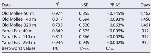
The model outputs appear to provide a generally good representation of water dynamics, but the evaluation parameters can help us quan-tify the extent of the fit. The detailed evaluation results chosen calibra-tion are listed in Table 3. Overall, the results are very good. The Pearson’sR2values, which are a measure of the linear fit between the model and piezometer data sets, are all>0.7 (with a value of 1 repre-senting a perfect fit). The NSE is a ratio of the residual to the data vari-ance (a value of 1 indicates equal variability in each), hence if the variability of the model output is within the scope of the piezometer variability then the NSE value shows good model performance. Hence, Old Mollee 320 m, with visibly less variability in model than piezome-ter data, has the poorest NSE value. Nevertheless, all NSE values were
>0.5.
The PBIAS values are a measure of the offset of the model data to the piezometer data. The results are all slightly negative, indicating an overestimation of model values, with the best results (closest to 0%) at the sites furthest from the channel and becoming poorer closer to the river. The Yarral East 110 and 290 m sites (Figures 5d and 5f) have the smallest PBIAS values. This can be attrib-uted to the model values being slightly above or slightly below piezometer readings in roughly equal mea-sures, hence the offset (drainage term) is optimal at these sites. The modulus of the PBIAS values at all sites were<0.15%. Overall, as expected, the Yarral East 290 m site performs best. The perceived worst performer in the visual comparison (Old Mollee 320 m) is substantiated by the results in Table 3.
4.2. Model Output
Time series of soil saturationHwithin a vertical slice of the floodplain, three distances from the river chan-nel, and across two different locations are exhibited in Figure 6. To understand the contribution of each flux (i.e., precipitation and lateral flow) to the soil, we can study soil-water patterns related to the following three categories: the phreatic zone (H51), the vadose zone (H<1), and interactions between the two zones. In the phreatic zone, the most apparent trend is that of reduced variability in the water table with distance from the river channel. In hydraulically connected floodplains, the water table is driven by river stage fluctu-ations that propagate and dissipate through the floodplain. Hence, the water table is less connected to the river channel with distance, making it less sensitive to changes in river water elevation and having the effect of smoothing the phreatic signal to remove extremes. Along with a dampening of the water table signal, there is a time delay, on the order of weeks. Peaks and troughs observed closer to the channel take time to propagate to the further sites, so rising and falling limbs are more gradual in the time series. There is also a very gradual decrease in average water table levels in the model output due to the positive drainage term.
Soil-moisture patterns in the upper part of the vadose zone are dominated by the surface flux. The climate inputs were the same for all six sites, so saturation patterns in the upper part are consistent. Soil saturation near the surface fluctuates, as heavy rains and evapotranspiration lead to saturated and dry soil-moisture extremes, respectively. The temporal legacy of individual rainfall events is exhibited in the angle of its infil-tration front as it progresses downward (see labeled infilinfil-tration on Figure 6e). Moving deeper into the soil, moisture fluctuations dampen and base soil saturation gradually increases. The increase in saturation is a result of slow infiltration rates, accumulating rainfall contributions, and the influence of the capillary fringe.
The capillary fringe below contributes soil-moisture to a significant depth interval of the vadose zone. The extent of this depth is influenced by the soil properties. This contribution is more visible at the near-stream sites (Figure 6a Mollee 50 m and Figure 6b Yarral 40 m), where capillary contributions from a higher water table interact more readily with the soil-moisture extremes from rainfall events. The capillary fringe moisture contribution is also more prominent at the further upstream Old Mollee sites, which have water table values at higher elevations and hence higher capillary fringes, than at Yarral East sites. It must be noted, however, that the floodplain surface elevation varies across the sites, which also affects the location of the water table with respect to the soil surface.
[image:12.630.46.306.139.230.2]At Old Mollee 50 m (Figure 6a) in early and mid-2012, the moisture in the capillary fringe connects with the infiltrating precipitation creating a region of very high saturation that reaches the surface. This underground connectivity, combined with high variability in water table levels, leads to a higher risk of flooding near the
Table 3
Results of the Statistical Tests Carried out on the Simulated Model Output Data Compared With the Observed Field-Measured Data
Data R2 NSE PBIAS Days
Old Mollee 50 m 0.974 0.855 20.145% 1,462 Old Mollee 140 m 0.817 0.694 20.093% 1,456 Old Mollee 320 m 0.735 0.520 20.063% 1,461 Yarral East 40 m 0.849 0.575 20.005% 912 Yarral East 110 m 0.811 0.566 20.002% 912 Yarral East 290 m 0.946 0.939 20.002% 912 Best/worst values 1/0 1/–1 0/1
river channel—irrespective of overbank conditions. Spikes in the water table due to capillary fringe connec-tion with infiltrating water also occur in early 2013 and 2014 but do not rise as far as the soil surface. Using this knowledge of increased connectivity in the vadose zone when the capillary fringe meets infiltrating water, we can look back at the model and piezometer comparisons (Figure 5), specifically at Mollee 140 m (c) and Mollee 320 m (e), and see that the under-prediction of water table peaks in early 2012 may be due to inaccuracies in the bulk soil properties used in the infiltration calculation (equation (2)). A higher satu-rated hydraulic conductivity in the vadose zone, for example, would lead to faster infiltration of rainfall events allowing them to connect with associated peaks in the capillary fringe. This exemplifies the impor-tance of the relationship between the vadose and phreatic zones for understanding patterns of water change in each.
4.3. Decadal Simulation
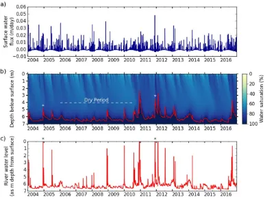
[image:13.630.90.548.98.461.2]Applying HaughFlow to a decadal time series allows us to investigate the response of soil-moisture distribu-tions to climatic fluctuadistribu-tions. Climate data from the Inverell Research Centre (station ID 94541099999, GSOD) provided a decadal time frame for the inputs. The Inverell Research Centre is located at229.78, 151.08 and has continuous data available from the beginning of 2003. Figure 7 shows the results of the lon-ger input series at the Old Mollee 140 m site from 2004 to 2017. Comparing the surface flux (Figure 7a) and river stage (Figure 7c) inputs with the soil saturation output (Figure 7b) allows us to fully examine the soil-moisture profiles and how each process drives changes. During the Australian summer months (December– February), patterns of heavy rainfall and strong evaporative drying are seen in Figure 7a, and replicated in
Figure 6.Saturation plots showing the upper 10 m of soil across the time series of sites at Old Mollee (left column), (a) 50, (c) 140, and (e) 320 m from the river
Figure 7b where they diffuse diagonally downward in time within the soil. River stage variations in Figure 7c are replicated in the water table (Figure 7b) with a time delay of approximately 24 days (which emerges directly from the Boussinesq equation, 140 m/Ks), and a reduced amplitude.
Comparing similar river stage peaks in late 2004 and late 2011 (asterisks in Figures 7b and 7c), the second peak is much more pronounced in the water table than the first. The only difference between the two being that soil-moisture levels were much higher deep in the soil preceding the second peak. Hence, river stage peaks are more pronounced in the water table when preceded by rainfall events that have infiltrated deep into the soil. There is a visible period of dryness in the soil, particularly for midrange depths from 2006 to mid-2010 (white dashed line in Figure 7b). Looking at Figure 7c, this dryness seems to be triggered by low river stage values from late 2005 to late 2008. Low rainfall in 2009 exacerbates this drying. This dry period matches the time frame of the southeast Australian ‘‘Millenium’’ drought (2001–2009), during which time groundwater storage was found to be particularly depleted from the end of 2006 until the beginning of 2010 (Van Dijk et al., 2013). Soil-moisture throughout the soil recovered in 2011 and 2012, which were very wet years due to a combination of high rainfall events and high river stage peaks.
The power of this model is its ability to quantify the water availability to rooting vegetation, in particular within dynamic and sensitive riparian environments, at different distances from the river. Plant species, depending on their rooting depths, may access different potential water reservoirs in the floodplain. To compare water availability for different plants at different locations, time series of water content was pro-duced over depth intervals. The soil-moisture was rescaled from saturationH(values range from 0 to 1), to a raw value of actual water contenthwithin a meter of soil (values range from the residual water contenthr,
to the saturated water contenths). Using the water content allows us to quantify the actual water available
[image:14.630.190.577.98.389.2]to vegetation rather than merely how filled the pore spaces are. In Figure 8, (a) Old Mollee 50 m, (b) Old Mollee 140 m, and (c) Old Mollee 320 m are compared. The plots show the water content in 1 m intervals down to 5 m. The saturated and residual water content for a 1 m depth range are provided as references for each plot.
Figure 7.(a) Plots showing the surface flux, (b) saturation profile, and (c) river stage time series for Old Mollee 140 m
The uppermost depth interval (0–1 m) at all the sites has the highest variability and contains the lowest overall levels of daily water content. Deeper-rooting vegetation has access to more water overall. The ‘‘0 m to 1 m’’ depth range is almost identical among all the three sites, yet differences become more pronounced moving deeper into the soil. The water content across all depths is high at Old Mollee 50 m, with near-complete saturation maintained within the 4–5 m depth. Saturation in this depth range indicates that the water table has risen to 4 m depth. The dry period identified between 2006 and mid-2010 in Figure 7 can be seen more clearly in the Old Mollee 140 and 320 m plots (Figures 8b and 8c). This is because the baseline water table depth is below 5 m for Old Mollee 140 and 320 m (see Figures 6 and 7b). So these depths are meters away from both the soil surface and the water table, making them more sensitive to periods of drought. When we compare the peaks in the 4–5 m water content in late 2010, late 2011, and early 2011 they decline more gradually in sites furthest from the river. This is because the water table further from the river is less variable. As water table levels are maintained for longer, the capillary fringe prolongs the decline to baseline water content levels. At the Old Mollee 320 m site, the capillary fringe allows water to be retained for up to months at 4–5 m deep. Hence, the water content just above the water table, further from the river is actually a much more reliable supply than above the water table nearer the river, which is more prone to daily fluctuation.
To further investigate the influence of the capillary fringe, we can observe the sharp difference in water con-tent in the peaks between 3–4 and 4–5 m depths in Figure 8c, indicating the excon-tent of the capillary fringe. Hence, the draw from the capillary fringe is not indefinite. Conversely, changes in water content moving down from the surface are more gradual, since water can continue infiltrating over time. Figure 9 allows us to examine these moisture patterns in a different way. Each column in the figure represents one of the Old Mollee sites, with histograms to the right representing sites further from the river.
[image:15.630.193.577.98.380.2]The shape of the histograms indicates the mean and variance in water availability for each depth interval. Bell-shaped curves (i.e., all three 0–1 m histograms: Figures 9a–9c) represent depths that are sometimes exposed to extremes of wet and dry water conditions. Right-skewed distributions (i.e., the 2–3 m soil depth at Old Mollee 50 m and the 4–5 m depth at Old Mollee 320 m: Figures 9g and 9o) have a consistent lower
Figure 8.The water content in 1 m depth intervals (h) down to 5 m for (a) Old Mollee 50 m, (b) Old Mollee 140 m, and (c)
threshold of water availability. The left-skewed distribution in Figure 9m portrays a depth with both high and consistent water availability. The highest water contents (all>70%) are located at 2–3, 3–4, and 4–5 m at the Old Mollee 50 m site and at 4–5 m at the Old Mollee 320 m site. The higher content at the Old Mollee 50 m site is because the water table is higher at this site (at4 m). The higher content at the deepest Old Mollee 320 m site is because of the low variability in the water table located a few meters below (at7 m deep). Hence, the water availability is higher and more reliable nearer the water table and further from the river channel. Depending on the water requirements and rooting depths of a particular plant species, plots like these could be used to analyze current, or plan future riparian plantations. Furthermore, climate projec-tions can be used to create these plots for future scenarios to investigate the water balance, soil-moisture, and vegetative water availability for a range of scientific and management applications.
5. Discussion
In this paper, we developed a new model with the capability to analyze coupled soil-moisture and water table fluctuations. Our model, HaughFlow, enables simple simulation of subsurface water fluxes in flood-plains, through dynamic coupling of lateral hyporheic flow and rainfall infiltration, based on existing theo-retical frameworks. We have coded this model in a manner that enables straightforward calibration of water table fluctuations and allows for decadal simulations of the impact of climate or even climate change on subsurface moisture. Water availability in catchments like the Murray-Darling basin are under increasing pressure from agricultural production and human use (Pittock & Connell, 2010). Having already experienced prolonged periods of drought, the majority of climate change scenarios foresee further water scarcity in the Murray-Darling region (Pittock & Connell, 2010). HaughFlow could be used to assess the impacts to water availability at multiple depths, and help inform water and ecological management plans.
Our application of HaughFlow to sites in southeast Australia identified a best approach for model calibra-tion. The model performed best when calibrated using piezometer sites furthest from the river. This is due to the propensity for otherwise underestimating floodplain connectivity with a low lateral hydraulic conduc-tivity value. We also showed the utility of the coupled-model approach, which significantly improves model performance. Further work is necessary to calibrate the unsaturated model component using high resolu-tion data on soil-moisture.
The model outputs demonstrate the importance of the interdependence of the vadose and phreatic zones. In the upward direction, the capillary fringe contributes to soil-moisture patterns and connectivity in the vadose zone; and downward, the temporal legacy of infiltrating water in the vadose zone manifests as increased water content stored deeper in the soil. High antecedent moisture conditions in the vadose zone can facilitate connection between rising and infiltrating waters, raising the water table. Hence, the capillary fringe is an important exchange pathway between the vadose and phreatic zones. The vadose zone pro-vides a significant store of water, particularly within the capillary fringe, which replicates fluctuations in the water table, and retains high levels of water saturation after peaks in the water table. This provides a critical moisture resource for shallow-rooting plants that are unable to reach the water table, which is particularly important further from the river channel.
Water table fluctuations became more delayed and less variable with distance from the river. At the furthest sites, delays in the propagation of river stage peaks are on the order of weeks, and the reduced variability means storage in the capillary fringe can maintain high water content for up to months. This storage poten-tially provides a valuable water resource to deeply rooting plants, particularly later in the dry season.
Water content over different depth ranges allow HaughFlow to be used for a range of scientific and man-agement applications relating to water and vegetation. If the rooting depths are known for a particular riparian species, then knowledge of the soil-water saturation over that depth can elucidate changes in the plant’s behavior. Of course, root-water uptake is not as simple as this, as is it challenging to accurately repre-sent root-water uptake with depth (Feddes et al., 2001) and plants can grow to adapt to their water avail-ability (Canham et al., 2012). For example, river red gum trees in the Murray-Darling Basin were found to adapt well to the ‘‘Millenium’’ drought (Doody et al., 2015). So for most effective results, HaughFlow should be used alongside knowledge of plant physiology.
The combination of different processes working in tandem within the riparian vadose and phreatic zones make floodplains highly dynamic in terms of hydrology and water availability to vegetation. To better understand the relative contributions of each process, further work could be done to decouple their inter-locking signals within the floodplain. One such way would be by delineating the capillary fringe. This is hard to do precisely, due to dynamic baseline soil-moisture conditions, no clear moisture threshold for the fringe, and unknown contributions from water infiltration. The incorporation of stable isotope tracers in HaughFlow could be used to establish water sourcing (Gat, 1996; Kendall & McDonnell, 2012). This would also make the model more powerful for use in vegetative water-use analysis, as plants take-up and store the stable isotopes from water at their rooting depths (Ehleringer & Dawson, 1992).
Appendix A: Numerical Methods
The numerical methods for the Richards equation and the Boussinesq equation are explained in the follow-ing subsections. A schematic of the physical and computational domains is shown in Figure A1.
The lateral domain extends from the river channel (x5W, grid pointi5nx) to the internal floodplain (x50,
grid pointi50). The computational grid points in the vertical domain are located at midlayers. Across both systems the vertical domain begins at the impermeable layer (z50, grid pointi521=2) up to the soil sur-face (z5H, grid point i5nz11=2). Richards equation can be applied to any position along the lateral
domain; in Figure A1 this is displayed as the midpoint on the lateral axis for simplicity. The spatial steps are
Dx5W=nxandDz5H=nz.
The boundary conditions in the model consist of:
[image:18.630.91.537.512.721.2]1. A prescribed flux (defined by the precipitation and surface evapotranspiration) atz5Hin the Richards equation.
Figure A1.Physical and computational domains used in the Richards equation (vertical) and in the Boussinesq equation (horizontal). NB: if there is no water table/
2. A specified hydraulic head (w52f5zwt) at the impermeable lower boundaryz50 in the Richards
equa-tion, or a zero flux condition if there is no water table within the modeled domain. 3. A prescribed river water elevation atx5Win the Boussinesq equation.
4. A zero flux condition at the far-channel extent of the Boussinesq equation.
The two equations are coupled through the water table. Specifically, the water table heightzwtðtÞprovides
the lower boundary condition in the Richards equation, while the flux at the water table boundary arising from the vadose zone provides the source termSin the Boussinesq equation. Details are given below.
A1. Initialization
The initialization of the water content throughout the vadose and phreatic zones is described herein. In equilibrium, with a constant level of waterhrin the river channel, and no external influences (including no
surface flux), the water table will eventually equilibrate laterally with the adjacent floodplain. This means the water level will become uniform throughout (hðx;0Þ5hr) and there will be no vertical flux. Hence, the
zero flux solutionfðz;0Þ5z2zwtin equation (9), withzwt5hrcan be applied throughout the domain.
A2. Richards Equation
Vertical water movement is simulated using the Richards equation (equation (2)) along with three equations forH(5),C(6), andK(7). For numerical simplicity, the following substitutions are applied to the three equa-tions whenf>0
Cs5akDh
s5ðafÞk
n5ð11afsÞ21:
(A1)
These lead to the following equivalent forms of equations (5)–(7)
H5nm
CðfÞ5CssHn
KðfÞ5KsH1=2ð12sHÞ2:
(A2)
Whenf0, the soil is saturated; there these functions simplify to the constantsH51,C50, andK5Ks.
These constants apply to the grid points below the water table.
Following Pikul et al. (1974), a tridiagonal formula along with a predictor-corrector scheme was used to evolve equation (2) in time. The main difference from Pikul et al. (1974) is in placing grid points at midlayer depths, as this simplifies the upper boundary condition. We also usefin place ofw.
The predictor step fromt5nDttoðn11=2ÞDtat each interior vertical grid point,i52,. . .,nz21, for equation
(2) uses the following discretization:
Cni f n11=2
i 2fni
ðDt=2Þ 5
Kn i11=2
Dz
fni1111=22f
n11=2
i
Dz 21
! 2K
n i21=2
Dz
fni11=22fni2111=2
Dz 21
!
; (A3)
where the grid-averaged conductivity term is defined byKi11=2521ðKi1Ki11Þ. Using the constants
r15
Dt
2Dz & r25 Dt
2Dz2; (A4)
we can rearrange this equation into tridiagonal form:
2r2Kin11=2f
n11=2
i11 1 Cni1r2Kin11=21r2K
n i21=2
fni11=22r2Kin21=2f
n11=2
i21
5r1 Kin21=22Kin11=2
1Cn ifni:
(A5)
With the solution forfni11=2, we can use equations (6) and (7) to obtain values forKin11=2 andCni11=2for
i51,. . ., nz. From Kn11
=2
i , we obtain K n11=2
i11=25ðK
n11=2
i 1K n11=2
i11 Þ=2 as before. Using Hn11
=2
nz , we can then
Cin11=2f n11
i 2fni
Dt 5
Kin1111==22
2Dz
fni11112fni11
Dz 21
2K n11=2
i21=2 2Dz
fni112fni2111
Dz 21
1K n i11=2 2Dz
fni112fni
Dz 21
2K n i21=2 2Dz
fni2fni21
Dz 21
;
(A6)
which we can rearrange as
2r2Kn
11=2
i11=2f
n11
i111 C
n11=2
i 1r2Kn
11=2
i11=21r2Kn
11=2
i21=2
fni112r2Kn
11=2
i21=2f
n11
i21
5Cni11=2fni1r1 Kn
11=2
i21=22K
n11=2
i11=21K
n i11=2
fni112fni
Dz 21
2Kn i21=2
fni2fni21
Dz 21
:
(A7)
When the water table is above the highest grid point in the domain, then flooding occurs. For flooding, no infiltration calculation is required and the surface flux is assigned at the water table boundary,Fwt5pr2er.
Evaporative fluxes can then diminish the water through the sink term in the lateral flow calculation until a vadose zone is formed (see Appendix A3.1 for more details on the calculation of the sink term).
A2.1. Lower Boundary
At the lowest grid point,i51, we make use of the bottom boundary conditionf52zwt. Takingfto be a
lin-ear function ofznearz50 then leads tof0522zwt2f1. This results in the following predictor and corrector equations:
2r2K3n=2f
n11=2
2 1 Cn11r2K3n=212r2K
n
1=2
fn111=2
5r1 K1n=22K3n=2
1Cn
1fn122r2DzK1n=2zwt;
(A8)
and
2r2Kn
11=2 3=2 f
n11 2 1 C
n11=2 1 1r2Kn
11=2 3=2 12r2K
n11=2 1=2
fn111
5r1 Kn
11=2 1=2 2K
n11=2 3=2 1K
n
3=2 fn22fn1
Dz 21
2Kn
1=2
2fn12zwt
Dz 21
1Cn
1f
n
122r2Kn
11=2 1=2 zwt:
(A9)
When the water table is below the lowest half-grid point (zwt<Dz=2), the domain is considered to be
unsaturated everywhere. In this case, a zero flux condition is applied atz50. For this case, the predictor step is
2r2K3n=2f
n11=2 2 1 C
n
11r2K3n=2
fn111=25C1nfn12r1K3n=2; (A10)
while the corrector step is
2r2Kn
11=2 3=2 f
n11 2 1 C
n11=2 1 1r2Kn
11=2 3=2
fn111
5Cn111=2fn12r1Kn
11=2 3=2 1r1K3n=2
fn22fn1
Dz 21
:
(A11)
A2.2. Upper Boundary
The upper boundary flux is calculated using the aforementioned daily precipitation rate (rp) minus the
evapotranspiration rate (re) (which is multiplied by the water contentHat the top boundary so it can never
exceed the available water). Thus, the surface fluxF5rp2reHnz. HereHnz is used in lieu ofHnz11=2to avoid
overshoots in extrapolation.
We use this given surface flux to simplify the equations near the upper boundary (i5nz). The predictor
step is
Cnnz1r2Knnz21=2
fn11=2
nz 2r2K n nz21=2f
n11=2
nz21 5C n nzf
n nz1r1ðF
n1Kn
nz21=2Þ; (A12)
Cnn1z1=21r2K n11=2
nz21=2
fnn11
z 2r2K
n11=2
nz21=2f n11
nz21
5Cnn1z1=2f n nz1r1 F
n11=21Kn11=2
nz21=21F n1Kn
nz21=2
fnn
z2f n nz21
Dz 21
:
(A13)
The model is able to simulate surface ponding both by precipitation rates exceeding the infiltration capacity and by the water table rising above the surface. The infiltration excess is evaluated by estimating the maxi-mum flux possible at each time step. Equation (10) is discretized numerically as
Fm5Ks 12
2fnz
Dz
; (A14)
where the pressure term (fnz) is located atz5H2Dz=2. If the input flux at the surface in the predictor or cor-rector step is greater than this maximum flux,F>Fm, then we add the excess,ðF2FmÞDt=2, to the
incom-ing flux at the next time step and set the current flux to the maximum,F5Fm. (NB: our unit of time is 1 day;
otherwise the excess would need to be divided by the length of the day to give a flux.) The ponding has not been limited in these simulations.
A3. Boussinesq Equation
We also use a predictor-corrector formulation for the Boussinesq equation, following Pikul et al. (1974) but using the variablebh2to solve equation (11) for all internal horizontal points,i, equally-spaced inx. Equa-tion (11) with thebsubstitution is
1
h
@b
@t5 Ks sy
@2b
@x212ðS2DrÞ: (A15)
The discretized predictor version of the equation is
Ks sy
bin1111=222bin11=21bni2111=2
Dx2 12ðS
n2D rÞ2
1
hn i
ðbni11=22bn iÞ
ðDt=2Þ 50: (A16)
The source/sink termSnis kept constant throughout the time step. Using the constant
r35
KsDt
2syDx2
; (A17)
we can rearrange the predictor step into the tridiagonal formula
r3hnib n11=2
i11 2 112r3hni
bni11=21r3hnib n11=2
i21 52ðSn2DrÞhniDt2bni: (A18)
The corrector step is
Ks
2sy bn11
i1122bn
11
i 1bn
11
i21
Dx2 1
bn
i1122bni1bni21
Dx2
12ðSn2DrÞ2
1
hni11=2 bn11
i 2bni
Dt 50 (A19)
which we can rearrange as
r3hni11=2bin11112 112r3hni11=2
bn11
i 1r3hin11=2bni2111
522ðSn2D
rÞhni11=2Dt2bni2r3hin11=2 bni1122bni1bni21
:
(A20)
At the near-river boundary,i5nx, a Dirichlet boundary condition is used to specify the height of the water
in the river channel ashnx5hrðtÞ. The predictor and corrector steps for the river boundary calculationi5nx
21 are the same as given in (A18) and (A20), after replacinghnxbyhrandbnxbyh
2
r.
The horizontal spatial extent of the model is chosen large enough so that the far-river boundary does not interfere with the water table dynamics in the area of interest near the channel. For this reason the far-river boundary, atx50 ori50 is specified to have a zero flux (or Neumann) boundary condition. For accuracy, nearx50,bis expanded in a quadratic polynomial. The quadratic Taylor/MacLaurin Series expansion ofhis
whereh0is the unknown value ofhatx50. Zero flux requires that atx50,
@h
@xðx50Þ50)a50: (A22)
We obtainh0from the known values ofhat grid pointsi51 and 2, giving
h05 4 3h12
1
3h2: (A23)
This term can then be used to replaceh0wheni51 in equations (A18) and (A20).
A3.1. Evaluating the Source/Sink Term
The source/sink term,S, is calculated by calculating the materials balance of the water in the domain. This calculation is carried out at the vertical evaluation site along thexaxis. As a default this is half way between the river channel and the inner-floodplain boundary. This simplification incurs some error because the extent of the vadose zone is defined by thex- dependent position of the water table. A more accurate solu-tion would calculate thex-dependent materials balance by calculatingS(x,t) throughout the lateral domain. This however would be more computationally intensive.
The materials balance calculation is defined by
S5change in vadose zone water content-change in the surface water input
time step3specific yield ; (A24)
where the change in vadose water content is calculated from
DhDzX
nz
i51
Hn11
i 2H n i
(A25)
in whichHni is the nondimensional soil saturation at the end of time stepnat grid pointi. The change in surface water input is
Dt
2 F
n1Fn11=2
(A26)
withFnrepresenting the incoming flux at time stepn. So the fluxF
wtat the top of the water table into the
phreatic zone is
Fwt5 DhDz
Dt Xnz
i51
Hn11
i 2Hni
21
2 F
n1Fn11=2
: (A27)
Finally, the source/sink term is the phreatic zone influx scaled by the capacity or specific yieldsyof the soil:
S5Fwt=sy: (A28)
Appendix B: Evapotranspiration Calculation
B1. Evapotranspiration Equation
The Penman-Monteith equation (Monteith, 1965; Penman, 1948) calculates the evapotranspiration rate as a function of the amount of energy incident on a region, the mass transfer gradient (wind and relative humid-ity), and the canopy conductance (for transpiration). The full equation is given by
ET5DðRns1RnlÞ1cKEqwkvvae
að12WaÞ
qwkv½D1cð11Cat=CcanÞ
: (B1)
HereDis the slope of the saturation-vapor versus temperature curve (kPa K21). The net radiation is calculated usingRnsandRnlwhich are the net shortwave and incoming longwave radiation, respectively (MJ m22d21).
In the second part of the numerator,cis the psychrometric constant (kPa K21). The remainder of this part calculates the mass transfer gradient using:KE, a coefficient that reflects the efficiency of vertical transport
of water vapor by the turbulent eddies of the wind (mkm21kPa21),qwwhich is the mass density of water
d21),e
athe saturation-vapor pressure at the air temperature (kPa) and,Wawhich is the relative humidity of
the air.
Finally, in the denominator,CatandCcanare the atmospheric and canopy conductances, respectively.
Equa-tion (B1) is based on the assumpEqua-tions that there is no ground-heat conducEqua-tion or water-advected energy, and heat-energy storage remains constant (Dingman, 2015). Appendix B2 describes the methods used to calculate each of the climate parameters from equation (B1), and Appendix B3 describes the calculation of the transpiration parameters.
B2. Climate Parameters
To calculate daily evaporation using equation (B1), the following parameters are required:D,Rns,Rnl,c,KE,
qw,kv,va,ea, andWa. These can be calculated using the latitude (/in decimal degrees) and altitude (zaltin
m) of the site along with the following climate values for a given dayndayof that year’s total number of
daysnyear(365 or 366): the maximum temperature (Tmaxin8C), the minimum temperature (Tminin8C), the
dewpoint temperature (Tdewin8C), the atmospheric pressure at the station (Pin kPa), the mean pressure at
sea level (P0in kPa), and the average wind speed (vain km d21). The equations presented below have been
sourced from Dingman (2015) unless stated otherwise.
The slope of the relationship between saturation-vapor pressure and temperature,D, can be calculated in kPa K21using the following equation:
D5 2508:3
ðTmean1237:3Þ2
exp 17:3Tmean
Tmean1237:3
; (B2)
whereTmeanis the average daily temperature in8C.
The methods for calculating the solar radiation have been taken from Allen et al. (1998). The net radiation incident on the surface in MJ m22d21is the sum of the net shortwave radiation,S, and incoming longwave radiation,L. First, we need the extraterrestrial radiation (Rain MJ m
22
d21), which is calculated using only the location of the site
Ra5
1440
p Gscdr½xssinðuÞsinðdÞ1cosðuÞcosðdÞsinðxsÞ (B3)
In this equation,Gscis a solar constant (0.0820 MJ m22min21),dris the inverse relative distance between
the Earth and Sun, calculated by
dr5110:033cos
2p 365nday
; (B4)
anddis the solar declination
d50:409sin 2p
365nday21:39
: (B5)
xsis the sunset hour angle, defined by the following equation:
xs5cos21½2tanðuÞtanðdÞ; (B6)
whereuis the latitude in radians.
The incoming solar radiation (Rsin MJ m22d21) can be inferred from this extraterrestrial radiation, along
with the maximum and minimum temperature readings, using the Hargreages and Samani [1982] radiation formula
Rs5kRs
ffiffiffiffiffiffiffiffiffiffiffiffiffiffiffiffiffiffiffiffiffi Tmax2Tmin p
Ra (B7)
which is a function ofkRs, an adjustment coefficient. Allen (1997) produced the following relation forkRs
kRs5kRa ffiffiffiffiffiffiffiffiffiffiffiffiffi
P=P0
ð Þ
p
; (B8)