Multi Value Sequence Generated over Sub Extension Field and Its Properties

(1)

ISSN Online: 2153-1242 ISSN Print: 2153-1234

DOI: 10.4236/jis.2019.103008 Jul. 2, 2019 130 Journal of Information Security

Multi-Value Sequence Generated over Sub

Extension Field and Its Properties

Md. Arshad Ali

1*

, Yuta Kodera

1

, Takuya Kusaka

1

, Satoshi Uehara

2

, Yasuyuki Nogami

1

,

Robert H. Morelos-Zaragoza

3

1_{Graduate School of Natural Science and Technology, Okayama University, Okayama, Japan}

2_{Faculty of Environmental Engineering, University of Kitakyushu, Fukuoka, Japan}

3_{Department of Electrical Engineering, San Jose State University, San Jose, CA, USA}

Abstract

Pseudo-random sequences with long period, low correlation, high linear complexity, and uniform distribution of bit patterns are widely used in the field of information security and cryptography. This paper proposes an ap-proach for generating a pseudo-random multi-value sequence (including a binary sequence) by utilizing a primitive polynomial, trace function, and k-th power residue symbol over the sub extension field. All our previous se-quences are defined over the prime field, whereas, proposed sequence in this paper is defined over the sub extension field. Thus, it’s a new and innovative perception to consider the sub extension field during the sequence generation procedure. By considering the sub extension field, two notable outcomes are: proposed sequence holds higher linear complexity and more uniform distri-bution of bit patterns compared to our previous work which defined over the prime field. Additionally, other important properties of the proposed mul-ti-value sequence such as period, autocorrelation, and cross-correlation are theoretically shown along with some experimental results.

Keywords

Pseudo-Random Sequence, Trace Function, Power Residue Symbol, Sub Extension Field, Autocorrelation, Cross-Correlation, Linear Complexity, Distribution of Bit Patterns

1. Introduction

Sequences of numbers generated by using an algorithm are referred to as a pseudo-random sequence. Pseudo-random sequences are inseparable parts in information technology as well as in modern electronics. They are used in both How to cite this paper: Ali, Md.A.,

Kode-ra, Y., Kusaka, T., UehaKode-ra, S., Nogami, Y. and Morelos-Zaragoza, R.H. (2019) Mul-ti-Value Sequence Generated over Sub Ex-tension Field and Its Properties. Journal of Information Security, 10, 130-154.

https://doi.org/10.4236/jis.2019.103008

Received: March 28, 2019 Accepted: June 29, 2019 Published: July 2, 2019

http://creativecommons.org/licenses/by/4.0/

(2)

DOI: 10.4236/jis.2019.103008 131 Journal of Information Security

communication (such as cellular telephones and GPS signals) and cryptographic applications (such as key stream for stream cipher, sampling data for simulations, timing measurements in radar systems, error correcting codes in satellite commu-nications, and so on). In most cases, it is important to have the reproduce ability of the pseudo-random sequence [1]. As well as it should have many desirable characteristics such as a long period, low correlation, uniformly distributed bit patterns, high linear complexity, and statistical randomness [2] to become a prominent candidate for information security and cryptographic related applica-tions [3] [4]. The randomness regarding a sequence is considered as the key strength of the cryptographic systems [5]. Considering this crucial point, it’s better to use some non-linear mathematical calculation during sequence generation. Ad-ditionally, the sequence must have randomness property. The major substance for randomness is independency of values (or lack of correlation), unpredictability (or lack of predictability), and uniform distribution (or lack of bias) [6]. Along with these, there are some statistical tests available to judge the randomness of a se-quence such as NIST, Diehard, ENT test [7]. It is mandatory to evaluate the ran-domness of a sequence before utilizing them in any cryptosystems.

Other geometric sequences having prominent pseudo-random properties are the Mersenne Twister (MT) [8], Blum-Blum-Shub (BBS) [9], Legendre sequence

[10], maximum length sequence (M-sequence) [11], and Sidelnikov sequence

[12]. Among those, the former two pseudo-random number generators (MT and BBS) are well known considering their applications in cryptography rather than the theoretical aspect. On the other hand, the latter sequences (Legendre sequence, M-sequence, and Sidelnikov sequence) are prominent geometric sequences re-garding the theoretical aspect. Generally, the typical features of a pseu-do-random sequence such as its period, correlation, linear complexity, and dis-tribution of bit patterns cannot be theoretically proven. However, if a sequence is defined over the finite field, then those features are often proven. All these above-mentioned sequences generated based on some mathematics more specif-ically they are defined over the finite field. Therefore, most of their important properties are already theoretically proven. The authors are basically more inter-ested in the theoretical aspects of a pseudo-random sequence rather than their ap-plications in the cryptographic area. Therefore, the authors motivated in this re-search work by observing the theoretical features of the well-known Legendre se-quence, M-sese-quence, and Sidelnikov sequence. Moreover, many researchers are also attracted by these theoretic aspects of these sequences. Our proposed sequence generated by the idea of the Legendre sequence and M-sequences, thus the authors thought that its properties can be theoretically proven and fortunately it proven.

Our previous work on binary sequence [13] uses a primitive polynomial, trace function, and Legendre symbol to generate a new variety of pseudo-random bi-nary sequence. In brief, the previous sequence generation procedure is as follows: firstly, it utilizes a primitive polynomial over an odd characteristic field p to

generate a maximum length vector sequence as elements in _pm, then applies

(3)

uses the Legendre symbol to binarize the scalars to binary sequence. Our previous binary sequence [13] generated by combining the features of M-sequence and L-sequence. Some important properties such as period, autocorrelation, and linear complexity have been theoretically proven in our previous work. Our previous works on multi-value sequence [14] [15] utilizes a primitive polynomial, trace function, and power residue symbol over odd characteristic field. Some important features of the sequence such as period, autocorrelation, and cross-correlation are theoretically proven in our previous work. The authors previous works on the binary sequence [13], signed binary sequence [16], and multi-value sequence

[15]are considered in the prime field p more specifically, the trace function

( )

Tr ⋅ _{maps an element of the extension field}_pm to an element of the prime

field p. Our previous work on multi-value sequence [17] considered on the sub extension field q characterized by four parameters however it has a shorter se-quence period of

(

1

)

. 1

m

k p n

q

− =

−

The period and autocorrelation properties of the proposed sequence explained based on some experimental results only.

The authors in this paper proposed a multi-value sequence (including a binary sequence) by applying a primitive polynomial, trace function, and k-th power residue symbol over the sub extension field q. The k-th power residue symbol is an extended version of the Legendre symbol. In details, the proposed mul-ti-value sequence generation procedure is as follows: let p be an odd characteris-tic prime and m be the extension degree of a primitive polynomial f x

( )

over the extension field _pm. It is well known that using the primitive polynomial

makes it possible to generate a maximum length vector sequence over _pm. Let

ω

be a zero of the primitive polynomial f x

( )

and it’s a primitive element in

m

p

∗

 . Then the sequence

( )

{

t ti| i Tr_{p q}m| ωi ,i 0,1,2, ,pm 2

}

= = =  −



becomes a maximum length sequence of having a period of _pm₋1_{, where,}

( )

|

Tr_{p q}m ⋅ is the trace function over the sub extension field q. It maps an

ele-ment of the extension field _pm to an element of the sub extension field _q.

After the trace calculation, a non-zero constant element A is added to the trace values. This non-zero A can be any arbitrary element within the sub extension field q such as A∈

{

1,2, , q−1

}

. Then, the k-th power residue symbol is

utilized for mapping the trace sequence



to a k-value sequence more specif-ically a multi-value sequence.

The authors recently started to consider the sub extension field q during

the sequence generation procedure, whereas, almost all our previous works on pseudo-random sequence [13][14] [15] are considered in the prime field p.

(4)

extension field _pm elements to prime field elements and the possible range of

trace outputs are

{

0p−1

}

. On the other hand, in case of sub extension field q

, the trace maps extension field _pm elements to sub extension field q elements and possible range of trace outputs are

{

0q−1

}

. Therefore, the sub extension field allows more variations in the trace values and from the theoreti-cal perspective, this flexibility contributes to the betterment of a sequence prop-erties. Thus, from this point of view it’s a new dimension in this research area. Some of the notable contributions of the authors in this paper are: this work is an extension of our previous works [13][14][15]; if the parameter k satisfies the condition k p|

(

−1

)

_{, then it also includes our previous work}_[15]_{; this work} overcomes the shorter period shortcoming of our previous work [17] by adding one more additional parameter A; the period, autocorrelation, and cross-correlation properties regarding the proposed sequence are explained both theoretically and experimentally; this work also makes a comparison in terms of autocorrelation, linear complexity, and distribution of bit patterns, according to the comparison results, it was found that the proposed sequence holds low correlation, high li-near complexity, and much better distribution of bit patterns compared to our previous work [14]. There are a lot of symbols used in this paper, thus a brief in-troduction about those symbols are introduced in Table 1.

2. Preliminaries

This section explains some fundamental concepts of the finite field theory such as a primitive polynomial, trace function, k-th power residue symbol, and dual basis. Then, multi-value sequence is introduced along with its properties such as period, autocorrelation, cross-correlation, linear complexity, and distribution of bit patterns.

2.1. Primitive Polynomial

Consider a polynomial f x

( )

of degree m over prime field p. If it is not fac-torized into smaller degree polynomials over the prime field p, it is called an irreducible polynomial. Consider the smallest number e such that _xe₋1_is

di-visible by f x

( )

over p, it is known that e becomes a factor of pm−1. Then

( )

f x is especially called a primitive polynomial, when e is equal to _pm₋1_{. Its} zero

ω

belongs to the extension field _pm and it becomes a primitive element

in _pm that generates every non-zero element in _pm as its power

ω

i (for

2

0,1,2, , m

i₌ _ p − _{). According to Fermat’s little theorem, the following property}

between _pm and its base field p holds [18].

Property 1. Let g be a generator of _p∗m, ( 1) ( 1)

q p

g − −

becomes a non-zero element in prime field p and is also a generator of p∗. □

2.2. Trace Function

This work utilizes the trace function to map an element of the extension field

m

p

(5)

[image:5.595.208.543.88.457.2]

Table 1. List of symbols used in this paper.

List of symbols p odd prime number

m positive integer, mainly denotes the extension degree

m′ one of the factors of m q power of the odd prime _{q p}₌ m′

k prime factor of q−1 such as k q|( −1)

p

 odd characteristic prime field m

p

 an extension field (base p and extension degree m)

q

 sub extension field

q

∗

 multiplicative group of q, excluding the 0 such as q q { }0

∗₌ ₋

  ( )

f x a primitive polynomial

ω root of an irreducible polynomial g generator of a group

A an arbitrary element in q

∗



( )

|

Tr_{p q}m ⋅ trace function maps _pm element to q element

k

 primitive k-th root of unity ( )

k

f ⋅ mapping function maps q element to k element

 proposed sequence in this paper n period of a sequence

( )

R ⋅ autocorrelation of a sequence 

( )

ˆ,

R_{ } ⋅ _{cross-correlation between the sequences} __and _ˆ

( )

1

|

0

Tr m im.

m m

p p q

i

x X X ′

− ′

=

= =

∑

(1)

A crucial point, the above trace becomes an arbitrary element in q and the

trace function has a linearity property over the sub extension field q as

fol-lows,

(

)

( )

| | |

Tr_{p q}m aX bY+ =aTr_{p q}m X +bTr_{p q}m Y , (2)

where a b, ∈q and X Y, ∈_pm. In this paper, the following property is

im-portant [18].

Property 2. For each arbitrary element α∈q, the number of elements in m

p

 whose trace with respect to q becomes

α

is given by p q pm = m m− ′ and the number of non-zero elements in _pm whose trace is zero is given by

(

_{p q}m

)

_{− =}1 _pm m− ′₋1_._□

2.3. k

-th Power Residue Symbol

(6)

DOI: 10.4236/jis.2019.103008 135 Journal of Information Security 1

q− as follows:

( )

( 1) 0

0, if 0,

1 , else if is a -th PR in , , otherwise is a -th PNR in , q k

k q

k

i

k q

a

a q a a k

a k

− ∗

∗

 =



= =_ =

 

  



(3)

where PR and PNR stand for Power Residue and Power Non-Residue respec-tively. The k is a primitive k-th root of unity that exists in q and 0≤ <i k. It becomes a Legendre symbol when k=2 [19] and if k p|

(

−1

)

, it becomes our previous work [15]. Note that, for a non-zero element a and a fixed k, the

exponent i in Equation (3) is uniquely determined in the range of 0k−1. Moreover, since k 0 ₁

k = k =

  and k is a prime number in this paper, the expo-nents can be dealt with as elements in k. This symbol is basically used for

checking whether or not a is a k-th PR over q as shown above. The output of the k-th power residue symbol can be represented as an exponent of k, where

k

 is a k-th primitive root. This paper uses k-th power residue symbol to trans-late a trace sequence over q to a k values multi-value sequence such as

{ }

0,ki ,

where i∈

{

0, ,_ k−1

}

_.

To represent the exponent i in Equation (3), this paper uses the following no-tations and it should be noted that the following notation excludes the case of

0

a= .

(

)

(

)

(

( 1)

)

log_k log_k q k . k

i₌ a q ₌ a −

  (4)

This paper utilizes the power residue symbol to map an element in q to an element in k. Regarding the power residue symbol

( )

a q k, the following property holds.

Property 3. For each i from 0 to k−1_{, the number of non-zero elements in} q

 such that

( )

i k k

a q = (5) is given by

(

q−1

)

k_.□

2.4. Dual Bases

Dual basis that is used for some proofs shown in this paper is defined as fol-lows:

Definition 1.Let _pm be a finite field and q be a finite extension of _pm.

Then the two bases =

{

α α0, , ,1 αm−1

}

and =

{

β β0, , ,1 βm−1

}

of q

over _pm are said to be the dual (or complementary) bases if

(

)

|

1, if , Tr

0, otherwise

m i j

p q

i j

α β =  =

 (6) where 1 ,≤i j m≤ −1. □

The dual basis of an arbitrary basis is uniquely determined in [18]. In this pa-per, the following property is important.

(7)

respectively. Based on the definition of dual basis and the linearity of the trace function, if

α

l be a basis of  in _pm is a non-zero sub extension field

ele-ment, then,

(

)

( )

| |

1, if ,

Tr Tr

0, otherwise,

m l j l m j

p q p q

j l

α β =α β =  =

 (7)

where 0 ,≤l j m≤ −1_{. Thus, when}

α

l =1, Tr_{p q}m_|

( )

β

l =1. □

2.5. Multi-Value Sequence and Its Properties

This paper introduces a k-value sequence, more specifically a multi-value se-quence as follows.

2.5.1. Notation and Period

Let multi-value sequence  is denoted as

{ }

s ii , 0,1,2, ,n 1,

= = _ − _

 (8)

where si∈

{

0,1, , k−1

}

and n be the period of the sequence such as s si = n i+ .

2.5.2. Autocorrelation and Cross-Correlation

The autocorrelation of a sequence is a scope for measuring how much the origi-nal sequence varies from its each shift value. After observing this property some special characteristic about the sequence can be found such as its period, some pattern of it, and so on [20]. The autocorrelation R

( )

x of sequence  shifted

by x is generally defined as follows:

( )

1

0

R n si x si, k i

x − + −

=

∑



  (9)

where k is a primitive k-th root of unity over the complex number . It

fol-lows that,

( )

1 0

0

R 0 n k .

i n

−

=

∑

 =

  (10)

The cross-correlation is as important as the autocorrelation property. It is calculated between two different sequences of having the same period and it ex-plains the sharing of some partial information between two sequences. In addi-tion, if multiple sequences are used in any application (such as in security appli-cation), in that case, it is important to analyze the similarities between those se-quences. To do so, the cross-correlation property needs to be evaluated. Consi-dering the security aspects, the value of the cross-correlation preferred to be low because the higher value of cross-correlation, the more similar the sequences to each other [21]. Let ˆ=

{ }

sˆ_i be a different sequence of having a period of n. Then, the cross-correlation at x shifted is generally defined by the following eq-uation as,

( )

1 ˆ

ˆ,

0

R n si x si, k i

x +

− −

=

∑



   (11)

(8)

2.5.3. Linear Complexity

The linear complexity (LC) of a sequence is closely related to how difficult it is to guess the next bit after observing the previous bits of a sequence. Since this pa-per considers k-value sequence with coefficients

{

0,1, ,_ k−1

}

_{, the linear} com-plexity of sequence  having a period of n is defined as follows.

( )

(

( )

)

LC _{= −}_n deg gcd _xn₋1,_{h x} ,



 (12)

where h x

( )

of =

{ }

si is defined over k as,

( )

1

0 .

n i i i

h x − s x

=

∑

 (13)

It should be noted that gcd

(

_xn₋1,_{h s}

( )

)

 in Equation (12) needs to be cal-culated over k, where k is a prime number and k q|

(

−1

)

. It is said that linear

complexity of pseudo-random sequence for security applications is preferred to be high.

2.5.4. Distribution of Bit Patterns

From the viewpoint of security, the distribution of bit patterns is as important as the linear complexity. If a sequence holds uniform distribution of bit patterns, then it becomes difficult to guess the next bit after observing the previous bit patterns. For example, let’s assume a binary sequence having a period of 12 as

{

}

12= 1,0,1,0,1,0,1,0,1,0,1,0

 . If we observe the 1-bit pattern in this sequence, then we can find that it has uniform distribution of 1 and 0. In other words, 1 and 0 appears same in number. However, when we check 2-bit patterns on 12, we find that it only has two type of patterns (10 and 01). In this case, we can eas-ily predict the next bit patterns after observing the previous patterns. Therefore, it is also essential to evaluate the distribution of bit patterns of a sequence to confirm its randomness.

3. Proposed Multi-Value Sequence

Let

ω

be a primitive element in the extension field _pm, n be the period of the

proposed multi-value sequence, m be a composite number which denotes the extension degree of the primitive polynomial, and m′_{be one of the factors of}

m. This paper proposes the following sequence  by utilizing the trace func-tion and k-th power residue symbol as follows:

{ }

i , i k

(

Tr_{p q}m_|

( )

i

)

.

k

s s f

ω

A p

= = +

 (14)

Here k is a prime number as well as a factor of q−1 such as k q|

(

−1

)

_{. To} make the above equation more simpler, from here on Tr_{p q}m_|

( )

⋅ will be represented

as Tr

( )

⋅ _{. Therefore, the above equation becomes,}

{ }

,

(

Tr

( )

i

)

.

i i k _k

s s f ω A p

= = +

 (15)

(9)

generated by the k-th power residue symbol to a multi-value sequence. The map-ping function fk

( )

⋅ is defined as follows:

( )

= 0,

₍

₎

if 0,

log_k , otherwise. k

k

x f x

x p

= 

  

(16)

As mentioned in Section 2.3, f xk

( )

with a fixed k maps an arbitrary element

q

x∈_ _{to an element in}__k_{. For example, by utilizing the parameter} p=5 and k=3_{, the sequence values will be in the range of}

{

0,1,2

}

, all of these val-ues are the elements of 3. In addition, let us fixed [1 4 3] be as a 3-rd primitive root of unity in q. Then, all of the sequence values can be represented as a

ex-ponent of this primitive root 3. More details of this example are shown in Ta-ble 2. This mapping function fk

( )

⋅ holds the following property.

Property 5. Consider x y, ∈q. If x≠0 and y≠0,

( )

1 _.

k k k

f x _± f y ₌ f xy±

(17)

Based on Section 2.3 and Property 3, the mapping function also satisfies the following equation, it should be noted that, here C is a non-zero element in q.

1

0 0.

k v k v

−

=

∑

 (18a)

( )

1

1 1 1

1 1 0

1 _0.

k k

p p _{f u} k

f u v

k k k

u u v

p k

−

− − −

= = =

−

 

= =_ _ =

 

∑



∑



∑

 (18b)

( )

1

1 1

1 1 0.

k k

p p _{f Cu}

f Cu

k k

u u

−

− −

= =

∑



∑

 (18c)

This section, firstly mathematically prove the cross-correlation property of the proposed multi-value sequence, then it explains the autocorrelation property, and finally the period is introduced. Additionally, these properties are also ob-served based on some experimental results.

3.1. Cross-Correlation

The cross-correlation is calculated between two different sequences of having the same period. These two different sequences ˆ and  can be defined as,

( )

(

)

{

}

ˆ _{ˆ ˆ}_| _Tr i _,

i i k _k

s s f ω B p

= = +

 (19a)

( )

(

)

{

| Tr i

}

.

i i k _k

s s f ω A p

= = +

 (19b)

Here, A and B are non-zero elements in q. They can be represented with a generator g that exists in the sub extension field q and they hold the following relation.

, h

B g A= ₍₂₀₎

(10)

[image:10.595.208.538.97.452.2]

Table 2. Mapping procedure of fk

( )

⋅ for 24 different trace Tr

( )

⋅ values1.

Output of Tr( )⋅ Output of (a p)k 3=[1 4 3] Output of fk( )⋅

1 [0] [3 1 2] [1 4 3]2 ₂

2 [1] [1 4 3] [1 4 3]1 ₁

3 [2] [3 1 2] [1 4 3] 2 ₂

4 [4] [1 4 3] [1 4 3]1 ₁

5 [0 1 2] [1] [1 4 3]0 ₀

6 [0 2 4] [1] [1 4 3]0 ₀

7 [0 3 1] [1 4 3] [1 4 3]1 ₁

8 [0 4 3] [3 1 2] [1 4 3]2 ₂

9 [1 1 2] [1] [1 4 3]0 ₀

10 [1 2 4] [3 1 2] [1 4 3]2 ₂

11 [1 3 1] [1] [1 4 3]0 ₀

12 [1 4 3] [3 1 2] [1 4 3]2 ₂

13 [2 1 2] [1] [1 4 3]0 ₀

14 [2 2 4] [1 4 3] [1 4 3]1 ₁

15 [2 3 1] [3 1 2] [1 4 3]2 ₂

16 [2 4 3] [1] [1 4 3]0 ₀

17 [3 1 2] [1] [1 4 3]0 ₀

18 [3 2 4] [3 1 2] [1 4 3]2 ₂

19 [3 3 1] [3 1 2] [1 4 3]2 ₂

20 [3 4 3] [1 4 3] [1 4 3]1 ₁

21 [4 1 2] [0] 0 0

22 [4 2 4] [1 4 3] [1 4 3]1 ₁

23 [4 3 1] [1 4 3] [1 4 3]1 ₁

24 [4 4 3] [1 4 3] [1 4 3]1 ₁

to be given by

ω

( )

pm−1 ( )q−1 , which used in the following proofs2_{. The}

cross-correlation of these two sequences ˆ and  is calculated as,

( )

1

(

Tr

( )

)

(

Tr

( )

)

ˆ,

0

R n fk i x g A fh k i A, k

i

x − ω+ + − ω +

=

∑



   (21)

where n is the period of these two sequences and according to the following sec-tion, it is given by _pm₋1_{. Furthermore, when} _h₌₀_{, then the value of}_A_and_B becomes exactly equal to each other, therefore, the cross-correlation becomes the autocorrelation of .

Theorem 1. The cross-correlation between the sequence ˆ and  given by Equation (21) is as follows.

( )

(

)

( )

(

)

(

)

(

)

( )

1 ˆ, 2

1 , if ,

R , else if ,

, otherwise,

h k

h j h j j h

k k k k

h k

f g

m m m m m

k

f A g g f A g f g f g

m m

k k k k

f g m m

k

p p p x hn

x p x jn

p − ′ ′ − − − − − ′ − ′ −  ₊ _{− −} ₌   _ _  =_ _ + − _− =     ₋                (22)

1_{In this example, we fixed [1 4 3] as a 3}rd_{primitive root of unity that exists in}

q

.

There-fore, every element can be represented as a power of this 3rd_{primitive root}

3

 . 2_Since _ω_{is a generator of}

m p

∗

 , therefore (_pm1)(_q1)

g ω − −

= becomes a generator of q

∗

(11)

where _{n n q}₌

(

_{− =}1

)

(

_pm₋1

)

(

_q₋1

)

_and_h_{satisfies the relation in Equation}

(20) as well as 0≤ ≠ ≤ −j h q 2. □

The proof for each case of Equation (22) is explained below. It should be noted that i holds the relation 0_{≤ < =}_{i n}

(

_pm₋1

)

_{and it is mainly appeared at}

summations. Furthermore, in the following section m m′_{is denoted as}_r_.

3.1.1. The Case of x hn=

In this case, the cross-correlation between the sequences ˆ and  becomes as follows:

( )

1

(

Tr

(

)

(

Tr

( )

)

1

(

Tr

( )

)

(

Tr

( )

)

ˆ,

0 0

R n fk i hn g A fh k i A n f gk h i A fk i A.

k k

i i

x − ω+ + − ω + − ω + − ω +

= =

=

∑

 =

∑



    (23)

According to Property 5 and depending on the condition of whether or not

( )

Tr

_ω

i _{+ =}_A 0_{, the above equation can be rewritten as follows:}

( )

(

)

(

Tr

)

(

Tr

( )

)

0 0 ˆ,

Tr =0 Tr 0

R k h k h i k i .

i i

g A f A

f g f

k k

A A

x ω ω

ω ω

+ − +

⋅ −

+ + ≠

=

∑

 +

∑



    (24)

Thus, the above equation becomes as,

( )

0 ˆ,

Tr =0 Tr 0

R k h .

i i

f g

k k

A A

x

ω + ω + ≠

=

∑

 +

∑



    (25)

It should be noted that _gh_≠0_{. Therefore, according to Property 2, the} cross-correlation between the sequence ˆ and  for the case of x hn=

holds the following relation.

( )

(

)

( )

ˆ,

R m m m 1 m m f gk h .

k

x ₌ p − ′₊ p _{− −}p − ′ _

   (26)

3.1.2. The Case of x= jn, j h≠

( )

1

(

Tr

(

)

(

Tr

( )

)

1

(

Tr

( )

)

(

Tr

( )

)

ˆ,

0 0

R n fk i jn g A fh k i A n f gk j i g A fh k i A.

k k

i i

x − ω+ + − ω + − ω + − ω +

= =

=

∑

_ =

∑

_

    (27)

According to Property 5, depending on the condition whether or not

( )

Tr

_ω

i _{+ =}_A 0_and _gj_Tr

( )

_ω

i ₊_{g A}h ₌₀_{following relation is obtained.}

( )

(

)

(

)

( )

(

)

(

)

( )

(

)

(

( )

)

1

1 ˆ,

Tr 0 Tr 0

Tr Tr

Tr 0 Tr 0

R

.

h j h j

k k

j i h j i h

i i

j i h i

k

j i h i

f A g g f A g

k k

g g A g g A

A A

f g g A A

k

g g A

A x ω ω ω ω ω ω ω ω − − − − − + ≠ + = + = + ≠   + +       + ≠ + ≠ = + +

∑

        (28)

For example, if Tr

( )

_ω

i _{+ =}_A 0_and _{j h}_≠ _{, then,}

( )

(

)

Tr 0.

j i h h j

(12)

re-DOI: 10.4236/jis.2019.103008 141 Journal of Information Security

spectively becomes as follows:

( )

(

)

(

)

(

)

Tr 0 Tr 0 ,

h j h j

k k

j i h i

f A g g _{m m} f A g g

k k

g g A

A p ω ω − ₋ _′ − + ≠ + = =

∑

  (30)

( )

(

)

(

1

)

(

1

)

Tr 0 Tr 0

,

h j h j

k k

j i h

i

f A g _{m m} f A g

k k

g g A

A p ω ω − − − − ₋ _′ − − + = + ≠ =

∑

  (31)

where the following facts and conditions should be noted for the above two summations:

 In this paper, the parameter A is not 0 and A∈q.

 The case of Tr

( )

_ω

i _{+ =}_A 0_, _gj_Tr

( )

_ω

i ₊_{g A}h _≠₀_.  While _gjTr

( )

_ω

i ₊_{g A}h ₌0_, _Tr

( )

_ω

i _{+ ≠}_A ₀_.

Assume, Tr

( )

i 0

i

X =

ω

+ ≠A _{. Then the third summation in Equation (28)}

becomes as follows:

( )

(

)

(

( )

)

( )

(

)

(

)

1 1 Tr Tr

Tr 0 Tr 0

.

j i h i _j _h _j

k _k _i

j i h j i h

i i

f g g A A _{f g} _{A g} _{g X}

k k

g g A g g A

A A ω ω ω ω ω ω − −  ₊ ₊    ₊ ₋     + ≠ + ≠ + ≠ + ≠ =

∑



∑

 (32)

Now all of the possible values of Xi∈q needs to be consider to resolve Eq-uation (32). According to Property 2 and considering the exceptions for the first and second summations in Equation (28), following relations are obtained,

{

}

# | 0 m m,

i

i X ₌ ₌ p − ′ _(33a)

(

)

{

}

# | 1 j m m,

i

i X ₌ A ₋g− ₌p − ′ _(33b)

{

}

# | m m 1,

i

i X ₌A ₌ p − ′₋ _(33c)

{

}

# | m m,

i

i X ₌u ₌ p − ′ _(33d)

here 0≤ <i n and for each _{u q}_{∈ −}

{

0, , 1_{A A}

(

₋_gh j−

)

}

_{. The cases of Equation}

(33a) and Equation (33b) respectively comply the first and second summations in Equation (28).

Furthermore, assume j

(

h j

)

1

i i

Y g₌ ₊A g ₋g X−

this is the input of mapping function fk

( )

⋅ as defined in Equation (32). Hence, considering the cases of

(

1 h j

)

i

X ₌A ₋g −

and Xi =0, the value of Yi in Equation (32) cannot be 0

and _gj_{, respectively. These two cases already separated in Equation (28) as the} first and second summations. As a consequence, Equation (32) can be rewritten as in Equation (34). In order to conform, the case of j

i

Y =g _{part (B) is added}

in Equation (34). Furthermore, part (C) in Equation (34) is for adjusting the number of cases of Xi =A, which mentioned in Equation (33c). Therefore,

(18b) holds at part A in Equation (34).

(13)

( )

(

)

(

)

( )

(

)

(

)

( )

(

)

(

)

( )

1 1 1 Tr 0 Tr 0 Tr 0 Tr 0 (B) (C) Tr 0 Tr 0

j h j

k i

j i h i

j h j

h h j j

k i

k k k k

j i h i

j h j j h

k i k k

j i h i

f g A g g X k

g g A A

f g A g g X f g f g _{m m} f g _{m m} f g

k k k k k

g g A A

f g A g g X _{m m} f g f g

k k k

g g A A p p p ω ω ω ω ω ω − − − + − + ≠ + ≠ + − ′ ′ − − + ≠ + ≠ + − ₋ _′ + ≠ + ≠     =_ − _{ }+ − _+     = + +

∑

                 

( )

(A) (A) 0 . j h k k

j h j h

k k k k

f g f g m m

k k

f g f g f g f g

m m m m

k k k k

p p p ′ − ′ ′ − −               − −     = − _ _− = − _ _−                 (34)

( )

(

)

(

)

( )

(

)

(

)

(

)

( )

1 ˆ, 1 R .

h j h j j h

k k k k

h j h j j h

k k k k

f A g g f A g f g f g

m m m m m m

k k k k

f A g g f A g f g f g

m m

k k k k

x p p p

p − − − − − ′ ′ ′ − − − − − − ′ − = + − −   = _ + − _−                

    (35)

3.1.3. Otherwise

( )

1

(

Tr

( )

)

(

Tr

( )

)

ˆ,

0

R n fk i x g A fh k i A. k

i

x − ω+ + − ω +

=

∑



   (36)

Here, x is not divisible by n and

_ω

x_{does not belongs to}

q

. We assume the following basis  in _pm, by using this

ω

x as,

{

ω

x,1, , , ,

γ γ

2 3

γ

r−1

}

.

= _

 (37)

Again let  be the dual basis of .

{

θ θ θ θ0, , , , ,1 2 3 θr−1

}

.

= 

 (38)

Assume that

_ω

i_{can be represented with}_θ_{as follows:} 1

,

0 .

r i

i l l l v

ω − θ

=

∑

(39)

Then,

_ω

i x+

is given by

1 ,

0 .

r

i x x

i l l l v

ω+ − θ ω

=

∑

₍₄₀₎

Based on Property 4, initial value of

_ω

i_{is as,}

( )

,1

Tr i .

i

v

ω

= ₍₄₁₎ As previously mentioned that,  and  are the dual bases to each other, therefore Tr

( )

_ω

i x+

(14)

( )

,0

Tr i x .

i

v

ω

+ ₌ ₍₄₂₎

After substituting these trace values, Equation (36) becomes as follows.

( )

1

(

,0

)

( ,1 )

ˆ,

0

R n f vk i g A f vh k i A. k

i

x − + − +

=

∑

_

   (43)

Based on Equation (18), the above equation is rewritten as,

( )

(

)

(

)

( )

,0 ,1

,0 ,0 ,0

,1 ,1 ,1

1 ,0 ,1 ,0 ,1 0 ˆ,

0 0 0

0 0 R . h k i k i

h h h

i i i

h

k i i

h i

i

f v g A

f v A

k k k

v g A v g A v g A

v A v A v A

f v g A v A

k

v g A

v A x − + − + + = + = + ≠ + = + ≠ + =  ₊ ₊      + ≠ + ≠ = + + +

∑

          (44)

According to Equation (18b) and

_ω

i_{holds the relation}₀_{≤ <}_{i n}_{, which}

ac-tually represents every non-zero element in _pm, therefore, the second and third

summations holds the following relations.

( ,1 )

,0 ,1 0 0 0. k i h i i

f v A

k

v g A

v A

− +

+ =

+ ≠

=

∑

 (45a)

(

,0

)

,0 ,1 0 0 0. h k i h i i

f v g A k v g A

v A

+

+ ≠

+ =

=

∑

 (45b)

In addition, by considering the sub extension field q and fixing the values of vi,0 and vi,1 the first summation holds the following relation as,

,0 ,1 0 2 0 0 . h i i m m k

v g A

v A

p − ′

+ =

+ = =

∑

 (45c)

Considering the same calculation procedure of Equation (34), the fourth summation in Equation (44) becomes as follows:

(

_,0

)

( _,1 )1

_{( )}

1

₍

₎

( )

,0 ,1

1 1 ₀ ₀

2 1 1 0 0 . h h

k i i k k k

h i

i

p p

f v g A v A _{m m} _{f ab} _f _{g A f} _A

k k k

a b v g A

v A p − ₋  ₊ ₊  − −   ₋ _′ + − +   = = + ≠ + ≠ = −

∑



∑∑

  (46)

Since

_ω

i_{cannot represent the zero vector, the number of vectors such that} ,0 0

i

v = _and vi_,1=0 is one less than that of the other combinations like

,0 0

i

v = _and vi_,1=1. That is why, the last subtraction

(

)

( )

0 h 0

k k

f g A f A k

+ − +



 is

re-quired in Equation (46). According to the condition from Equation (18b), the first summation in Equation (46) becomes 0. Therefore, the following relation is obtained,

(

)

( )1

_{( )}

,0 ,1 ,0 ,1 0 0 . h h

k i i _k

h i

i

f v g A v A f g

k k

v g A v A −  ₊ ₊      + ≠ + ≠ = −

∑

  (47)

Therefore, the cross-correlation of the sequences ˆ and  becomes as follows for this case,

( )

2

( )

ˆ,

R m m f gk h .

k

x ₌ p − ′₋_

(15)

Finally, the cross-correlation of the sequences ˆ and , that is in Equation (22), is proven.

3.2. Autocorrelation and Period

If the value of h=0_{, then} ˆ and  becomes the same sequence. In this case, the cross-correlation in Equation (22) becomes the autocorrelation after replac-ing the value h=0_.

( )

(

( )

1

)

(

1

)

( )

2

1, if ,

R 1, else if ,

1, otherwise.

j j j

k k k

m

f A g f A g f g

m m

k k k

m m

p x hn

x p x jn

p

−

− − −

′ −

 − =



 



=_ _ + − _− =

 



 ₋



  

    (49)

Corresponding to the above autocorrelation equation, the period of the pro-posed multi-value sequence explicitly given by _pm₋1_.

4. Examples and Discussions

This section experimentally observes the properties of the proposed sequence such as period, autocorrelation, and cross-correlation along with some examples. Throughout this section, x provides the absolute value of a complex number

x. In addition, the notation 3 denotes the proposed sequence with the para-meter A=3.

4.1. p

=

5,

m

=

4,

m

′

=

2,

k

=

2 and

A=3,4

Let _{f x}

( )

₌_x4₊₂_x3₊₂_x2₊₂_x₊₂_{be a primitive polynomial over} 5

 . In this case, the period of this sequence becomes _pm_{− =}1 624_{. Then the sequence}

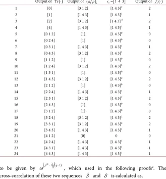
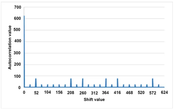
[image:15.595.210.539.493.708.2]

3  is shown in Equation (50) and its autocorrelation becomes as follows and Figure 1 shows its autocorrelation graph.

(16)

{

3 001000111010000000100000000110101001100011001001101110101011

010100001001001010000101001001101000110000100001110101101010 010000100000110111011110100111101100000010110001000001111001 10010010000110000

= 

1001011110111011110001110111001010001110101 111100100111000110011000000011110000111110110000111110110110 000001101100011101000011100101010100111110001000100001110011 011110010110111010101000101110010000111001001101010100011111 010100001011101011010110111101101010001110000010010111101000

}

100101101101111010100000100001011001001001100001110000110000 111111110101010101100110110110111110100011010011111101100110 001001101100101001100110

(50)

( )

3

624, if 0

24, else if 26,78,104,130,156,182,234,286,312,338,390,442,468,494,520,546,598, R

76, else if 52,208,260,364,416,572, 0, otherwise

x x x

x

= 

 ₌



=  ₌

  

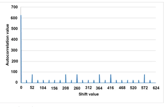
(51) On the other hand, it should be noted that 4 is different from 3 and its autocorrelation is given as follows and Figure 2 shows its autocorrelation graph.

( )

4

624, if 0

24, else if 26,78,104,130,56,182,234,286,312,338,390,442,468,494,520,546,598, R

76, else if 52,208,260,364,416,572, 0, otherwise

x x x

x

= 

 ₌



=  ₌

  

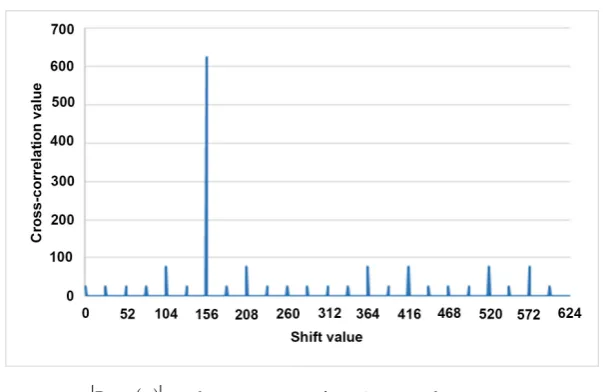
(52) The cross-correlation of 3 and 4 becomes as follows and Figure 6 shows its cross-correlation graph.

( )

3 4,

24, if 0,26,52,78,130,182,234,260,286,312,338,390,442,468,494,546,598, 76, else if 104,208,364,416,520,572,

R

624, else if 156, 0, otherwise

x x x

x

= 

 ₌



=  ₌

   

(53)

4.2. p

=

7,

m

=

4,

m

′

=

2,

k

=

3 and

A=3,4

Let _{f x}

( )

₌_x4₊₄_x3₊₃_x2₊₅_x₊₃_{be a primitive polynomial over} 7

 . In this case, the period of the sequence becomes _pm_{− =}1 2400_._{Figure 3}_,_{Figure 4}_,

and Figure 5 show the autocorrelation graphs of 3 , 4 , and the

cross-correlation between the 3 and 4, respectively.

By observing the experimental results, it is found that in every case, the cross-correlation graph has exactly q−1 number of peaks. Among those, only one has a maximum value. For example, in Figure 6, the maximum cross-correlation value is 624, which corresponds to the first case of x hn= _{, the}

(17)

[image:17.595.219.530.50.741.2]

Figure 2. R4

( )

x with p=5,m=4,m′=2,k=2, and A=4.

[image:17.595.221.530.61.258.2]

Figure 3. R3

( )

x with p=7,m=4,m′=2,k=3, and A=3.

[image:17.595.223.524.289.484.2]

(18)

[image:18.595.222.529.64.253.2]

Figure 5. R 3 4,

( )

x with p=7,m=4,m′=2,k=3, and A=3,4.

Figure 6. R 3 4,

( )

x with p=5,m=4,m′=2,k=2, and A=3,4.

these q−1 peaks the remaining part in the graph always holds a constant value of 0, which corresponds the case third case in Equation (22). It means that all this cross-correlation graph can be explained by Equation (22). It is also ob-served that by changing all the parameter values does not have any impact in the cross-correlation evaluation. On the other hand, as like the cross-correlation, the autocorrelation graph also has q−1 number of peaks. Among them, only one holds the maximum value, the others have small values, the remaining part al-ways holds a constant value of 1, and all these autocorrelation graphs can be ex-plained by Equation (49).

5. Comparison with Previous Work

[image:18.595.222.524.284.480.2]

(19)

Even though the authors proposed sequence is a multi-value sequence. but it can be easily mapped into binary sequence by setting the parameter value k=2_{. In} this section the authors will introduce a comparison of their proposed sequence (binary case) with their previous work [14] in terms of autocorrelation, linear complexity, and distribution of bit patterns properties. In this section, the authors previous sequence proposed in [14] will be called as NTU (Nogami-Tada-Uehara) sequence.

5.1. Autocorrelation

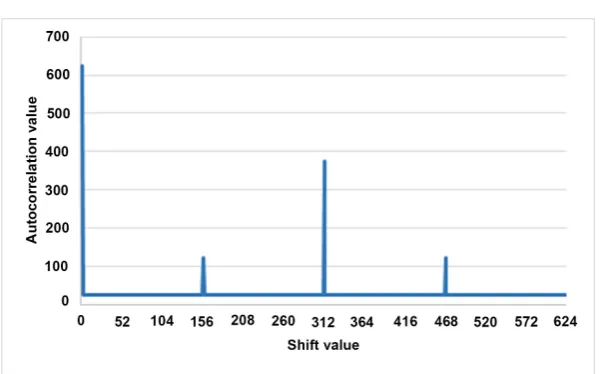
The autocorrelation of a sequence is a measure for how much the sequence dif-fers from its each shift value. In addition, by evaluating this property some spe-cial characteristics about the sequence such as its period, some pattern of the sequence, and so on can be also found and the value of the autocorrelation al-ways preferred to be as low as possible [22]. The autocorrelation of the proposed sequence (defined over sub extension field) and our previous sequence (NTU) (defined over prime field) is shown in Figure 7 and Figure 8, respectively. By observing their autocorrelation graph, it was found that on one hand, the num-ber of peak values is increases in the sub field sequence, on the other hand, the difference between the maximum peak value with the smaller peak values are much smaller in the proposed sequence compared to our previous sequence. Moreover, in the proposed sequence except the peaks remaining autocorrelation value always remains at 0. It should be noted that in case of correlation evalua-tion, the less difference between the peak values are more crucial rather than the number of peaks [22].

5.2. Linear Complexity

[image:19.595.223.528.520.709.2]

The unpredictability of a sequence can be measured by the length of the shortest Linear Feedback Shift Register (LFSR) which can generate the given sequence. This approach is particularly appealing since there exists an efficient procedure

(20)

[image:20.595.224.528.62.249.2]

Figure 8. Autocorrelation of NTU sequence.

(it is so called the Berlekamp-Massy algorithm [23]) for finding the shortest LFSR. This length is referred as the linear complexity associated with the se-quence. The linear complexity property regarding a sequence is an important parameter which tells how difficult it is to predict the next bit pattern by ob-serving the previous bit pattern of a sequence. Thus, the linear complexity of a sequence is always preferred to be high. The linear complexity of the proposed sequence (defined over sub extension field) and our previous sequence (NTU) (defined over prime field) is shown in Figure 9 and Figure 10, respectively. By observing their linear complexity graph, it was found that the proposed sequence (which defined over the sub extension field) always hold high linear complexity compared to the NTU sequence. In other words, in terms of linear complexity the sequence defined over the sub extension field hold higher linear complexity than the sequence defined over the prime field.

5.3. Distribution of Bit Patterns

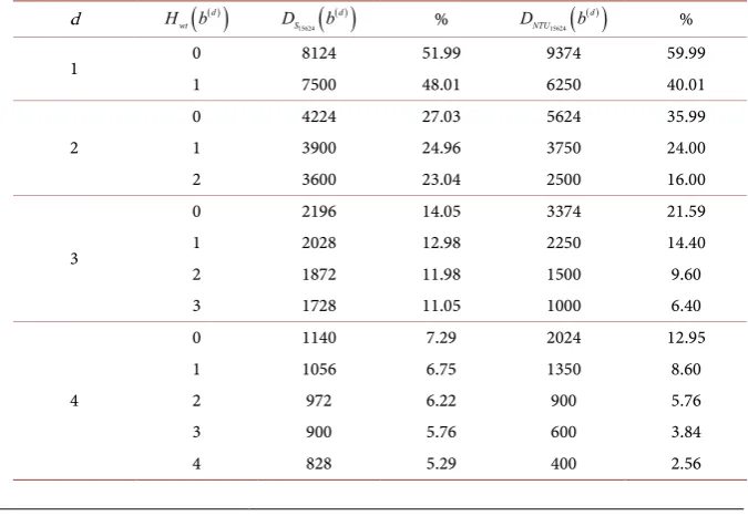
The distribution of bit patterns is another important measure to check the ran-domness of a sequence. From the viewpoint of security, the distribution of bit patterns is as important as the linear complexity. If a sequence holds the uniform distribution of bit patterns, then it becomes difficult to guess the next bit after observing the previous bit patterns. After the experimental observation, it was found that the NTU sequence is not uniformly distributed. In other words, in case of binary NTU sequence, there is much difference in appearance between the 0 and 1. To improve this drawback, instead of prime field (which used in the NTU sequence generation procedure), the authors focused on the sub extension field during the sequence generation procedure in this research work. As a result, after utilizing the sub extension field, the distribution of bit patterns becomes close to uniform. This comparison is shown in the following Table 3. In the fol-lowing table, _b( )d _,

( )

( )d

wt

H b , and _{D b}_n

( )

( )d

 denotes a bit pattern b of length d,

(21)

[image:21.595.221.530.62.243.2]

[image:21.595.223.525.274.449.2]

Figure 9. LC of the proposed sequence.

Figure 10.LC of the NTU sequence.

Table 3. Comparison in bit distribution between the sub field binary sequence and NTU sequence.

d

( )

( )d wt

H b

( )

15624

d S

D b %

( )

15624

d NTU

D b %

1 0 8124 51.99 9374 59.99

1 7500 48.01 6250 40.01

2

0 4224 27.03 5624 35.99 1 3900 24.96 3750 24.00 2 3600 23.04 2500 16.00

3

0 2196 14.05 3374 21.59 1 2028 12.98 2250 14.40

2 1872 11.98 1500 9.60

3 1728 11.05 1000 6.40

4

0 1140 7.29 2024 12.95

1 1056 6.75 1350 8.60

2 972 6.22 900 5.76

3 900 5.76 600 3.84

[image:21.595.201.539.508.741.2]

(22)

DOI: 10.4236/jis.2019.103008 151 Journal of Information Security ( )n

b , respectively. In terms of the distribution of bit patterns, the sequence de-fined over the sub extension field hold much better distribution (close to uni-form) of 0 and 1 than the sequence defined over the prime field.

As mentioned previously, NTU sequence proposed in [14] is defined over the prime field and proposed sequence in this paper is defined over the sub exten-sion field. After the comparison results it is concluded that in terms of correla-tion the proposed sequence holds low correlacorrela-tion compared to NTU sequence; about linear complexity proposed sequence possesses high linear complexity than NTU sequence; regarding the distribution of bit patterns proposed se-quence hold much better distribution of bit patterns (close to uniform) than NTU sequence.

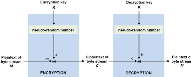
One of the most common applications of the pseudo-random binary sequence is in a stream cipher. Basically, stream cipher is divided into two classes: block cipher and stream cipher. Among these in case of block cipher, same key is used for both encryption and decryption of each block (≥64 bits) of data. On the oth-er hand, in case of stream ciphoth-er, encryption and decryption are poth-erformed by the bit wise ⊕ (XOR) operation with a key stream. Here, the authors restrict the discussion of their proposed pseudo-random binary sequence in a stream cipher. An image of the stream cipher is shown in Figure 11. Few important considerations during the design of a stream cipher are the key (which used for both encryption and decryption) should have large period, good randomness, and unpredictability properties due to the usage of same key in both encryption and decryption. Here, the encryption is carried out by applying a bit-wise ⊕

(XOR) operation between the plain-text of byte stream M and encryption key K. Then, the cipher-text C transmitted through a network. On the other hand, during the decryption, after the bit-wise ⊕_{operation between the cipher-text}

C and the same key K we will get the original plain-text M. In a stream cipher, a lot of sequences are assigned to several users, respectively. If these sequences have some correlation, then it will make some security vulnerabilities. Under this circumstance, it is important to observe the cross-correlation property be-tween several sequences. Additionally, its linear complexity and distribution of bit patterns needs to be high and uniform, respectively to confirm its random-ness. The authors proposed method can generate a long period pseudo-random sequence with typical auto and cross-correlation, high linear complexity, and almost uniformly distributed bit patterns features. After observing the experi-mental and comparison results, it can be concluded that the authors proposed sequence which defined over the sub extension field can be a prominent candi-date for a stream cipher like applications.

6. Conclusions and Future Works

(23)

[image:23.595.208.534.75.206.2]

Figure 11. Application of the proposed sequence in stream cipher.

research work are as follows:

 This is an extension of our previous works [13][14][15].

 _{This work overcomes the shorter period shortcoming of our previous work}

[17].

 The period, autocorrelation, and cross-correlation properties regarding the proposed sequence are theoretically explained.

 The authors make a comparison in terms of autocorrelation, linear complex-ity and distribution of bit patterns properties with their previous work [14].

 According to the comparison results, the proposed sequence holds low cor-relation, high linear complexity, and much better distribution of bit patterns compared to our previous work [14].

 The proposed sequence can be a prominent candidate for stream cipher like cryptographic applications due to its exemplary properties.

As future works, the following points should be researched:

 Mathematically prove the linear complexity and distribution of bit patterns properties.

 _{To introduce more efficient calculation instead of the power residue}

calcula-tion.

Acknowledgements

This work has been supported by JSPS KAKENHI Grant-in-Aid for Scientific Research (A) Number 16H01723.

Conflicts of Interest

The authors declare no conflicts of interest regarding the publication of this pa-per.

References

[1] Goresky, M. and Klapper, A. (2012) Algebraic Shift Register Sequences. Cambridge

University Press, Cambridge.

[2] Hamza, R. (2017) A Novel Pseudo Random Sequence Generator for Image-Cryptographic

Applications. Journal of Information Security and Applications, 35, 119-127.