Analysis of the Manufactured Tolerances with the Three Dimensional Method of Angular Chains of Dimensions Applied to a Cylinder Head of Car Engine

Analysis of the Manufactured Tolerances with the

Three-Dimensional Method of Angular Chains of

Dimensions Applied to a Cylinder Head of Car Engine

Aida Mezghani1,2, Alain Bellacicco2, Jamel Louati1, Alain Rivière2, Mohamed Haddar1

1_{Mechanics Modelling and Production Research Unit, ENIS, TUNISIA}

2_{Laboratoire d’Ingénierie des Structures Mécaniques et des Matériaux, SUPMECA Paris, FRANCE}

E-mail: [email protected]

Received May 4, 2010; revised July 21, 2010; accepted August 16, 2010

Abstract

This paper proposes an analysis method of the manufactured tolerances applied to a cylinder head of car en-gine. This method allows to determine the manufacturing tolerances in the case of angular chains of dimen-sions and to check its correspondence with the functional tolerances. The objective of this work is to analyze two parameterized functions: the angular defect Δα and the projected length lg of the toleranced surface. The angular defects are determined from the precision of the machine tools, we consider only the geometrical defects (position and orientation of surfaces), making the assumption that the form defects are negligible. The manufactured defect is determined from these two parameterized functions. Then it will be compared with the functional condition in order to check if the selected machining range allows, at end of the manu-facturing process, to give a suitable part.

Keywords:Three-Dimensional Tolerancing, Manufacturing Process, Toleranced Surface, Angular Defect.

1. Introduction

Today, the manufacturing engineers face the problem of selecting the appropriate manufacturing process (ma-chining processes and production equipments) to ensure that design specifications are satisfied. Developing a suitable process is complicated and time-consuming.

To verify the capacity of a manufacturing process to make the corresponding parts it is necessary to simulate the defects that it generates and to analyze the corre-spondence of produced parts with the functional toler-ances. In order to check the capability of a manufactur-ing process to carry out suitable parts, it is necessary to analyze each functional tolerance. In the literature avail-able on this subject, the evaluation of a process in terms of functional tolerances is called the tolerance analysis, [1-5].

The best way to analyze the tolerances is to simulate the influence of parts deviations on the geometrical re-quirements. Usually, these geometrical requirements limit the gaps or the displacements between product surfaces. For this type of geometrical requirements, the influences of parts deviations can be analyzed by different

ap-proaches as Variational geometry [6,7], Vectorial toler-ancing [8,9], Clearance space and deviation space [10- 13], Gap space [14], quantifier approach [15,16], kine-matic models [17,18], Inertial Tolerancing [19].

In this paper the three-dimensional method of angular chains of dimensions is used for simulating the manu-facturing process and then manufactured torerancing is determined to carry out tolerance analysis

2. Description of the Method

The three-dimensional method of angular chains of di-mensions, initiated by [20], allows the optimization of the calculation of three-dimensional angular dispersions. This method also allows the validation of the manufac-turing range by taking into account the processes preci-sion.

that the form defects are negligible. The manufactured defect is first determined from these two parameterized functions. Then it is compared with the functional condi-tion in order to check if the selected machining range allows, at the end of the manufacturing process, to give a suitable part.

2.1. The Angular Defect

The angular defect can be determined through two methods: the 2D method used currently in the industries and the new 3D method, in order to compare the results given by both methods.

2.1.1. 2D Approach

To determine the angular defect of a surface with the 2D method, it is necessary to choose two projection plans (perpendicular to the toleranced surface). Then the angu-lar defect in each plan is determined by the 1D method of angular chains of dimensions. The angular defect of the toleranced surface is given by the combination of both angular defects found in the analysis plans.

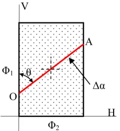
If the angular chains of dimensions are made in two projection plans (H and V for example), perpendicular between them, the defect in the plan V lies between zero and an angle 1. It will combine with a defect,

manufac-tured in the plan H, located between zero and 2.

The greatest angular defect Δαmax, resulting from the

combination of the two defects, is given by:

max

Δα 2 2

1 2

= Φ

+

Δαmax is located in the direction which forms an angle θ

with the plan V.

2 1

( / )

Atan F F

 (2) The diagram of the angular defects is shown in Figure 1. Referring to this diagram, the angular defect Δα is given in each analysis direction in accordance with θ. The value of the angular defect is equal to the length of the segment OA.

Figure 1. Diagram of the angular defects (2D method).

2.1.2. 3D Approach

In reality, the normal vectorsn, of the various machined surfaces, is contained in a volume forming a conical zone of tolerance. These zones of tolerance constitute solid angles.

The method consists in cumulating the solid angles which represent the angular defects of the part’s surfaces in the aim of finding the angular defect of the toleranced surface.

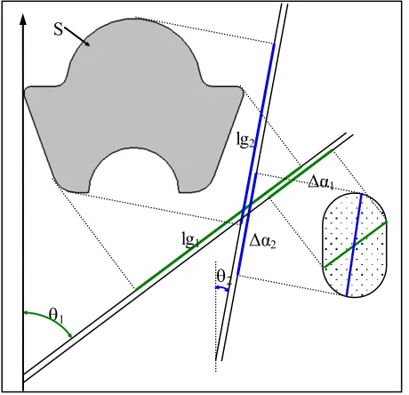
For a given machining range, it is necessary to deter-mine the locus of each manufactured defect, from the 1st phase until the nth phase. The combination of these de-fects gives a solid angle comparable to a right cone with an oblong form directrix. The manufactured defects dia-gram will have an oblong form instead of a rectangular one.

A parameterized diagram is drawn on a CATIA file related to a table of parameter setting. This parameter setting makes it possible to change the shape of the dia-gram according to the machine precision and the orienta-tion of posiorienta-tioning surfaces (Figure 2).

Referring to this diagram, the angular defect Δα is given in each analysis direction in accordance with θ. The value of the angular defect is equal to the length of the segment BC. To determine the value of Δα the CA-TIA macros are used. For each value of θ, Δα is meas-ured then transferred towards an EXCEL file.

2.2. The Manufactured Defect

The manufactured defect tf is the greatest height meas-ured between the toleranced element, surface S consid-ered plane, and the associated exact theoretical plan.

The measured defect tf is given by the Equation (3)

 

 

 

tf     lg  (3) with

Δα(θ): the angular defect of the toleranced surfaces in each analysis plan.

lg(θ): the projected length of the toleranced surface in each analysis plan.

When S surface has a particular form (Figure 3), the projected length lg is not uniform in all the analysis di-rections. To determine the various values of the projected length according to θ we use software CATIA. The val-ues of lg are extracted from the CAD model of the part. The projected surface length is measured for each value of θ then automatically transferred from CATIA towards an Excel file. Then we obtain a table which contains all the values of lg for a sweeping of θ.

The projected length and the angular defect Δα are given for a sweeping of θ then the manufactured defect tf can be deduced. tfmax will be compared with the func-tional condition.

3. Case Study: A Cylinder Head of Car

Engine

In this paper, the studied example is a cylinder head of car engine. The functional geometrical conditions of orien-tation are checked by using the method of three-dimen-sional angular chains of dimensions.

The geometrical orientation conditions, such as paral-lelism, perpendicularity and angularity will be treated in order to check their respect according to the machining processes precision.

Figure 4 represents the Digital Mock-Up (DMU) of the cylinder head made with the geometrical orientation conditions to study.

Digital Mock Up or DMU allows real-time visualiza-tion of the complete product in 3 dimensions and to de-scribe it during its life cycle. The DMU is a virtual ver-sion of the product that makes it possible to create all the

1

S

lg1

Δα1

Δα2

lg2

2

Figure 3. Case of particular form surface.

Figure 4. Digital Mock-Up (DMU) of the cylinder head with the orientation geometrical conditions.

simulations needed for product development, manufac-turing and the aftermarket.

The DMU enables the simulation of the product with the intention of knowing future and to replace the physi-cal prototypes with the virtual ones.

The cylinder head machining range comprises three phases. Table 1 summarizes them. This table highlights the manufactured and positioning surfaces in each phase.

We will study the feasibility of the DD condition: par-allelism of H relative to R-S. The angular defect is de-termined by the 2D method then the 3D or the spatial method.

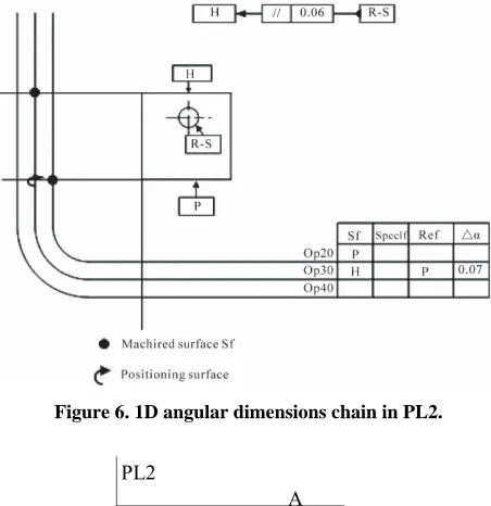
The precision of the used machine is 0.007 mm. This corresponds to an angular defect Δα = 0.07 mrd for 100 mm length and in any direction.

Table 1. Machining range of the head cylinder.

Operation Positioning surfaces Machined _surfaces

OP 20 W V Y P

P V Y H and HH

P V F’ J

P J F’ K

OP30

P K Y F and G

P K F A-B

P 542 _{(cylindrical pins)} A (milled pins)

601-610

P 542 _{(cylindrical pins)} 515 (milled pins)

Spot-facing 601-610 OP40

P 542 _{(cylindrical pins)} 515 (milled pins)

3.1. The Angular Defect

3.1.1. 2D Approach

In order to determine the angular defect generated by the manufacturing process, in each projection plan, we use the 1D angular chains of dimensions.

The machining range proposed for the cylinder head manufacturing indicates that the toleranced surface is machined before the reference element, which explains the need for a tolerances transfer.

Figures 5 and 6 show the 1D dimensions chains plot on the projection plans (PL1 Parallel to G and F, PL2 Parallel to K and J).

The cumulated defect in the projection plan can be deduced from this chain of dimensions:

- in PL1 the cumulated angular defect is Δα = 0.14 mrd. - in PL2 the cumulated angular defect is Δα = 0.07 mrd. Then the diagram of the angular defect is represented in Figure 7 with 1 = 0.07 mrd and 2 = 0.14 mrd.

Referring to this diagram the angular defect Δα can be given in each analysis direction in accordance with θ. The value of the angular defect is equal to the length of the segment OA. So we obtain the result of Figure 8 which represents the angular defect Δα in each analysis direction.

According to this result the maximum angular defect is 0.155 mrd. It’s located in the analysis direction which has θ = 1.11 rd

This result can be found using calculation since

max

Δα 2 2

1 2

= Φ

+

3.1.2. 3D Approach

To determine the resulting angular defect, it’s necessary to cumulate the solid angles and the plan angles which represent the angular defects of the manufactured sur-faces.

Figure 5. 1D angular dimensions chain in PL1.

Figure 6. 1D angular dimensions chain in PL2.

θ 0.07

0.14

PL1 PL2

A

O

Figure 7. The angular defect diagram (2D Method).

the angular defect Δα according to θ

0 0,02 0,04 0,06 0,08 0,1 0,12 0,14 0,16 0,18

0 0,5 1 1,5 2 2,5 3 3,5

θ (rd)

Δα

(mrd

)

Figure 8. The angular defect of the toleranced surface ac-cording to . (2D method).

The defect associated to the toleranced surface (nor-mal vector z) is modeled by a solid angle which the directrix diameter depends of the precision of the ma-chine. The direction vector for R-S is x, therefore only the angular defect of rotation according to y is consid-ered. The angular defect of rotation according to zdoes not have influence on the respect of the parallelism con-dition.

Table 2. Directrix of the cumulated defect.

phase Manufactured _surface

Locus of the manufactured

defect

Directrix of the cumulated defect

30 H Angle solide

Cercle Ø 0.07

40 R-S Angle plan

Oblong 0.140.07

Figure 9 presents the diagram of the angular defect Δα given by the 3D method. The manufactured defects dia-gram has an oblong form instead of a rectangular form.

Referring to this diagram the angular defect Δα can be given in each analysis direction in accordance with θ. The value of the angular defect is equal to the length of the segment BC. We obtain the result of Figure 10 which represents the angular defect Δα in each analysis direction.

The greatest defect is equal to 0.14 mrd. It’s located in the analysis direction which has θ = 1.57 rd. It is noticed that the angular defect determined by the 3D approach is smaller than the angular defect found by the 2D method. After that we will use the results of Figure 8 and Figure 10 to determine the manufactured tolerances in both cases and to compare them with the functional specifica-tions.

3.2. The Manufactured Defect

The method requires geometrical data relative to the tol-eranced surface. These data are extracted from the CAD model of the cylinder head. Figure 11 represents the form of the toleranced surface.

We use CATIA to determine the projected length in each analysis direction that is shown in Figure12.

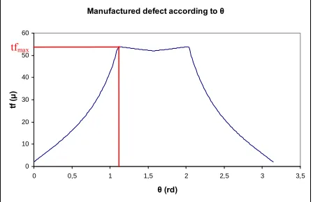
To determine the critical defect, it is necessary to ex-press the measured defect tf according to the two inde-pendent variables: the angular defect Δα(θ) and the pro-jected length lg(θ). Figure 13 and Figure14 present the manufactured defect determined respectively by the 2D method and 3D method.

The result of Figure 13 shows that the maximum manufactured defect is equal to 0.067 mm. It’s exceeded the limits imposed by the functional requirement (paral-lelism of 0.06 mm according to R-S). So the used ma-chine cannot satisfy the parallelism condition. We must use a more precise machine. This increases the produc-tion cost of the part.

V

H Δα

B

C

θ

Figure 9. The angular defect diagram (3D Method).

The angular defect Δα according to θ

0 0,02 0,04 0,06 0,08 0,1 0,12 0,14 0,16

0 0,5 1 1,5 2 2,5 3 3,5

θ (rd)

Δα

(m

rd

)

Figure 10. The angular defect of the toleranced surface according to . (3D method)

Figure 11. Form of the toleranced surface.

The projected length according to θ

0 50 100 150 200 250 300 350 400 450 500

0 0,5 1 1,5 2 2,5 3 3,5

θ (rd)

lg

(

m

m

)

Figure 12. The projected length of the toleranced surface according to .

Manufactured defect according to θ

0 10 20 30 40 50 60 70 80

0 0,5 1 1,5 2 2,5 3 3,5

θ (rd)

tf

(

μ

)

tfmax

Figure 13. The manufactured defect of the toleranced sur-face (H) according to  (2D method).

Manufactured defect according to θ

0 10 20 30 40 50 60 70

0 0,5 1 1,5 2 2,5 3 3,5

θ (rd)

tf

(

μ

)

tfmax

Figure 14. The manufactured defect of the toleranced sur-face (H) according to  (3D method).

The 3D method allows to optimize the manufactured tolerance intervals and to check the feasibility of the parts according to the machine precision. We will be able to choose a less precise machine and to reduce the pro-duction cost.

Next we present the results for several orientation

con-ditions. The same methodology is used to check the cor-respondence of these conditions with the functional specifications according to the machine precision.

Condition 2: parallelism of R-S relative to datum sur-face P.

In this case the toleranced element is machined di-rectly relative to the datum surface P. it doesn’t need a tolerance transfer. At worst the manufactured tolerance must be equal to the value of the tolerance interval of the DD requirement (0.04 mm). The parametric function lg(θ) is a constant equal to the length of the axis R-S. As a result, the precision machine needed to satisfy the func-tional specification is of p = 0.097 mm.

Condition 3: parallelism of HH relative to datum axis R-S.

Figure 15 and Figure 16 present the manufactured defect determined respectively by the 2D method and 3D method for p = 0.007 mm.

Both methods show that the use of a machine, which precision is 0.007 mm, makes it possible to satisfy the functional specification (parallelism of 0.055 mm rela-tive to R-S).

Manufactured defect according to θ

0 10 20 30 40 50 60

0 0,5 1 1,5 2 2,5 3 3,5

θ (rd)

tf

(

μ

)

tfmax

Figure 15. The manufactured defect of the toleranced sur-face according to  (2D method).

Manufactured defect according to θ

0 10 20 30 40 50 60

0 0,5 1 1,5 2 2,5 3 3,5

θ (rd)

tf

(

μ

)

tfmax

- 2D method: tfmax = 0.052 mm

- 3D method: tfmax = 0.054 mm

Condition 4: parallelism of the melts of spot facing relative to the datum surface P.

The toleranced element is machined directly relative to the datum surface. Only the defect generated by the ma-chining of the toleranced element is considered. Conse-quently, the diagram of the angular defect determined by the 2D and 3D method has respectively a square form and a circular form.

The toleranced surface has a circular form, so lg (θ) is constant and equal to the diameter of the surface, which explains the result of the Figure 18. The manufactured defect is a constant for any value of θ.

Figure 17 and Figure 18 present the manufactured defect determined respectively by the 2D method and 3D method for p = 0.45 mm.

The DD condition is checked only with the 3D method. This method allows the optimization of the choice of the machine compared to the 2D method.

We notice that the precision p = 0.45 mm is justified by tow facts:

Manufactured defect according to θ

0 20 40 60 80 100 120 140 160

0 0,5 1 1,5 2 2,5 3 3,5

θ (rd)

tf

(

μ

)

tfmax

Figure 17. The manufactured defect of the toleranced sur-face according to  (2D method).

Manufactured defect according to θ

0 20 40 60 80 100 120

0 0,5 1 1,5 2 2,5 3 3,5

θ (rd)

tf

(

μ

)

tfmax

Figure 18. The manufactured defect of the toleranced sur-face according to  (3D method).

- The dimensions of the toleranced surface are smaller than the dimensions of the other toleranced surfaces studied previously.

- The toleranced element is machined directly relative to the datum surface

Condition 5: perpendicularity of G relative to the da-tum axis R-S.

In the same way, the condition of perpendicularity is analyzed. Figure 19 and Figure 20 present the manufac-tured defect determined respectively by the 2D method and 3D method for p = 0.01 mm.

We find the following results: - 2D method: tfmax = 0.052 mm

- 3D method: tfmax = 0.037 mm

The result find with the 3D method shows that the condition of perpendicularity of G relative to R-S can be respected if p = 0.01 mm

It is noticed that dimensions of the toleranced surfaces have a great influence on the choice of the machine. It is always delicate to respect the tight tolerance interval relative to large-sized toleranced surfaces.

Table 3 summarizes the results find with the 3D method.

Manufactured defect according to θ

0 10 20 30 40 50 60

0 0,5 1 1,5 2 2,5 3 3,5

θ (rd)

tf

(

μ

)

tfmax

Figure 19. The manufactured defect of the toleranced sur-face according to  (2D method).

Manufactured defect according to θ

0 5 10 15 20 25 30 35 40

0 0,5 1 1,5 2 2,5 3 3,5

θ (rd)

tf

(

μ

)

tfmax

Table 3. Summary of the results.

DD condition

Form and di-mension of the toleranced sur-face

Manufactured defect find with the 3D method

Machine precision

Condition 1 Rectangular form

151  411.5 mm

tfmax = 0.058

mm p = 0.007 mm

Condition 2 _Axis 411.5 mm

tfmax = 0.04

mm p = 0.097 mm Condition 3

HH 0.055 R-S

Common zone Rectangular _form 371.5 27 mm

tfmax = 0.054

mm p = 0.007 mm

Condition 4 _{Circular form}

22 mm

tfmax = 0.099

mm p = 0.45 mm

Condition 5 Rectangular form 150  113 mm

tfmax = 0.037

mm p = 0.01 mm

The machining of surfaces H and HH requires a more precise machine compared with the other part surfaces. That is explained by two reasons: on the one hand, the tolerance intervals of the functional specifications are too tight; on the other hand, the toleranced surfaces have larger dimensions. Moreover, in both cases, toleranced surfaces are not machined directly relative to the datum. Consequently the accumulation of the defects generated in each phase of the manufacturing range increases the manufactured defect.

4. Conclusions

In this paper, we have presented a three-dimensional method of manufactured tolerances analysis applied to a cylinder head of a car engine. This method makes it pos-sible to evaluate the validity of a manufacturing process and to analyze the defects which occur in the various production phases. The use of CATIA macros decreases considerably the processing time of the examples and facilitates the treatment of the geometrical conditions.

We showed here an example of a cylinder head of a car engine in which we can see that the choice of the machine precision depends on the dimensions of the tol-eranced surfaces and the interval of tolerance required by the Design Department. This method is not a specific one, but a general one. It can be used in the case of industrial complex examples.

5. References

[1] F. Germain, D. Denimal and M. Giordano, “A Method for Three Dimensional Tolerance Analysis and Synthesis Applied to Complex and Precise Assemblies,” in IFIP International Federation for Information Processing, Vol-ume 260, Micro-Assembly Technologies and

Applica-tions, Springer, Boston, 2008, pp. 55-65.

[2] F. Villeneuve and F. Vignat, “Manufacturing Process Simulation for Tolerance Analysis and Synthesis,” Pro-ceedings of IDMME, 2004, Bath, 10 pages.

[3] M. H. Kyung and E. Sacks, “Nonlinear Kinematic Toler-ance Analysis of Planar Mechanical Systems,” Computer Aided Design, Vol. 35, No. 10, 2003, pp. 901-911. [4] R. J. Gerth and W. M. Hancock, “Computer Aided

Tol-erance Analysis for Improved Process Control,” Interna-tionl Journal of Computers and Industrial Engineering, Vol. 38, No. 1, 2000, pp. 1-19.

[5] Z. Shen, G. Ameta, J. J. Shah and J. K. Davidson, “A Comparative Study of Tolerance Analysis Methods,” Journal of Computing and Information Science in Engi-neering, Vol. 5, No. 3, 2005, pp. 274-284.

[6] J. Hu, G. Xiong and Z. Wu, “A variational Geometric Constraints Network for a Tolerance Types Specifica-tion,” International Journal of Advanced Manufacture Technology, Vol. 24, No. 3-4, 2004, pp. 214-222. [7] U. Roy and B. Li, “Representation and Interpretation of

Geometric Tolerances for Polyhedral Objects,” Computer Aided Design, Vol. 31, No. 4, 1999, pp. 273-285.

[8] J. Y. Dantan, J. Bruyere, J. P. Vincent and R. Bigot, “Vectorial Tolerance Allocation of Bevel Gear by Dis-crete Optimization,” Mechanism and Machine Theory, Vol. 43, No. 11, 2008, pp. 1478-1494.

[9] E. Ballot and P. Bourdet, “A Computation Method for the Consequences of Geometric Errors in Mechanisms,” Proceedings of CIRP Seminar on Computer Aided Tol-erancing, Toronto, Canada, April 1997, pp. 197-207. [10] M. Giordano, S. Samper and J. P. Petit, “Tolerance Analysis

and Synthesis by Means of Deviation Domains, Axi- Symmetric Cases” of the 9th CIRP International Seminar on Computer Aided Tolerancing, Tempe (US), April, 2005, pp. 85-94.

[11] A.Mujezinovic, J. K. Davidson and J. J. Shah, “A New Mathematical Model for Geometric Tolerances as Ap-plied to Polygonal Faces,” Transaction of the ASME, Journal of Mechanical Design, Vol. 126, No. 4, 2004, pp. 504-518.

[12] J. P. Petit, S. Samper and M. Giordano, “Minimum Clear-ance for TolerClear-ance Analysis of a Vacuum Pump,” Pro-ceedings of the 8th CIRP seminar on computer aided de-sign, Chalrotte (US), 2003, pp. 43-51.

[13] S. Bhide, G. Ameta, J. K. Davidson and J. J. Shah, “Tol-erance-Maps Applied to the Straightness and Orientation of an Axis” of the 9th CIRP International Seminar on Computer Aided Tolerancing, Tempe (US), April 2005, pp. 45-54.

[14] Z. Zou and E. P. Morse, “A Gap-Based Approach to Capture Fitting Conditions for Mechanical Assembly,” Computer Aided Design, Vol. 36, No. 8, 2004, pp. 691 -700.

[16] S. Tichadou, O. Legoff and J. Y. Hascoet, “Quantifica-tion of Machining and Fixture Errors: 3d Method and Analysis of Planar Mechanical Systems,” Computer Aided Design, Vol. 35, No. 10, 2003, pp. 901-911.

[17] E. Sacks and L. Joskowicz, “Parametric Kinematic Tol-erance Analysis of Planar Mechanisms,” Journal of Com-puter Aided Design,Vol. 29, No. 5, 1997, pp. 333-342.

[18] M. Kyung and E. Sacks, “Nonlinear Kinematic Tolerance Analysis of Planar Mechanical Systems,” Computer Aided Design, Vol. 35, No.10, 2003, pp. 901-911. [19] M.Pillet, “Inertial Tolerancing,” The Total Quality

Maga-zine, Vol. 16, No. 3, 2004, pp. 202-209.