Toric Heaps, Cyclic Reducibility, and Conjugacy in Coxeter Groups

(1)

ISSN Online: 2161-7643 ISSN Print: 2161-7635

DOI: 10.4236/ojdm.2019.94010 Sep. 18, 2019 110 Open Journal of Discrete Mathematics

Toric Heaps, Cyclic Reducibility, and Conjugacy

in Coxeter Groups

Shih-Wei Chao

1

_{, Matthew Macauley}

2

1_{Department of Mathematics, University of North Georgia, Dahlonega, GA, USA} 2_{School of Mathematical and Statistical Sciences, Clemson University, Clemson, SC, USA}

Abstract

In 1986, G.X. Viennot introduced the theory of heaps of pieces as a visualiza-tion of Cartier and Foata’s “partially commutative monoids”. These are es-sentially labeled posets satisfying a few additional properties, and one natural setting where they arise is as models of reduced words in Coxeter groups. In this paper, we introduce a cyclic version of a heap, which loosely speaking, can be thought of as taking a heap and wrapping it into a cylinder. We call this object a toric heap, because we formalize it as a labeled toric poset, which is a cyclic version of an ordinary poset. Defining the category of toric heaps leads to the notion of certain morphisms such as toric extensions. We study toric heaps in Coxeter theory, because a cyclic shift of a reduced word is simply a conjugate by an initial or terminal generator. As such, we formalize

and study a framework that we call cyclic reducibility in Coxeter theory,

which is closely related to conjugacy. We introduce what it means for ele-ments to be torically reduced, which is a stronger condition than simply being cyclically reduced. Along the way, we encounter a new class of elements that we call torically fully commutative (TFC), which are those that have a unique cyclic commutativity class, and comprise a strictly bigger class than the cycli-cally fully commutative (CFC) elements. We prove several cyclic analogues of results on fully commutative (FC) elements due to Stembridge. We conclude with how this framework fits into recent work in Coxeter groups, and we correct a minor flaw in a few recently published theorems.

Keywords

Conjugacy, Coxeter Group, CFC, Cyclic Reducibility, Faux CFC, Cyclically Fully Commutative, Heap, Logarithmic, Morphism, TFC, Torically Fully Commutative, Toric Heap, Toric Poset, Toric Reducibility, Trace Monoid

How to cite this paper: Chao, S.-W. and Macauley, M. (2019) Toric Heaps, Cyclic Reducibility, and Conjugacy in Coxeter Groups. Open Journal of Discrete Mathe-matics, 9, 110-143.

https://doi.org/10.4236/ojdm.2019.94010

Received: May 28, 2019 Accepted: September 15, 2019 Published: September 18, 2019

(2)

DOI: 10.4236/ojdm.2019.94010 111 Open Journal of Discrete Mathematics

1. Introduction and Overview

In mathematics and computer science, a trace is a set of strings or words over an alphabet S for which certain pairs are allowed to commute. The commutativity

rules can be encoded by an undirected graph Γ called the dependency graph,

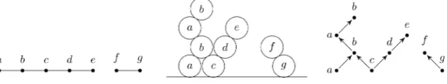
where the vertices are the letters and edges correspond to non-commuting pairs. Given a trace, the associated trace monoid is the set of finite words under the equivalence relation generated by these commutations, where the binary opera-tion is concatenaopera-tion. The combinatorics of trace monoids were studied by Car-tier and Foata in the 1960s, who called them partially commutative monoids [1]. They are now sometimes known as Cartier-Foata monoids. We will stick with the term “trace monoid” for brevity. In 1986, G. X. Viennot [2] introduced the theory of heaps of pieces, which is a combinatorial interpretation of these objects that leads to a nice way to visualize them. The “pieces” represent the distinct let-ters in the alphabet, and a string is represented by a vertical stack, or “heap” of these pieces. Two pieces overlap vertically if the corresponding letters do not commute, as elements in the monoid. A simple example of this follows.

Example 1.1. Consider the trace monoid *

S over the alphabet

{

, , , , , ,

}

S

=

a b c d e f g

with dependency graph Γ shown on the left in Figure 1.

That is, two letters commute if and only if they are non-adjacent in Γ_{. The}

string acbabgdfe in S* defines a heap of pieces shown in the middle of

Fig-ure 1. One can think of this as being built by dropping balls in a “Towers of

Hanoi” fashion onto this dependency graph—pieces of the same type are aligned vertically, and two pieces of different types overlap vertically if they do not commute. This heap (of pieces) is just a labeled poset (sometimes called its ske-leton), whose Hasse diagram is shown on the right in Figure 1. Note that every “labeled” linear extension is a string that gives rise to the same heap.

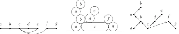
Trace monoids can be defined for arbitrary graphs, though the visualization of the heap in Figure 1 works well because Γ_{is a line-graph. For more complicated} planar graphs, we might need to make the pieces oddly shaped for the “Towers of Hanoi” visualization to work, which originally motivated Viennot’s heaps of pieces. For example, in Figure 1 the piece c does not commute with either b

or d. If we want to further require that it does not commute with e and f , one way to represent this is to elongate it, as shown in Figure 2. The new depen-dency graph and Hasse diagram of the labeled poset are shown as well.

[image:2.595.213.538.638.699.2]

For more complicated dependency graphs Γ_{, e.g. non-planar ones, the labeled} poset arising from a trace monoid over Γ does not have a nice visual realization

Figure 1. The dependency graph Γ_{of a trace monoid (left), a heap of pieces (middle),}

(3)

[image:3.595.221.531.73.132.2]

DOI: 10.4236/ojdm.2019.94010 112 Open Journal of Discrete Mathematics Figure 2. This heap of pieces is created from the heap in Figure 1 by additionally re-stricting c from commuting with e andf . This adds new edges to the dependency

graph and new relations to the poset.

in 2- or 3-dimensional space as a stack of pieces. However, there is still an un-derlying labeled poset which we can rigorously formalize as a heap. In Section 3, we will formally define all terms so there is no ambiguity about our notation. However, in the remainder of this section, we will assume a few basic definitions that the reader likely already knows, so we can summarize the outline, goals, and main ideas of this paper.

Since Viennot introduced them in 1986, heaps have been defined in various ways, depending on the context, and usually with the “of pieces” dropped from

the name. The following definition is due to R.M. Green [3], who defined the

category of heaps and applied it to Lie theory. Having a category makes defini-tions like a subheap and a morphism between heaps both natural and precise, and we will revisit this in Section 3.

Definition 1.2. A heap is a triple

(

P

, ,

Γ

φ

)

consisting of a poset P, a graph

Γ_{, and a function}

φ

:

P

→ Γ

to its vertex set, satisfying:

1) For every vertex s of Γ, the subset φ−1

( )

{ }

_s is a chain in _P, called a

vertex chain.

2) For every edge

{ }

s t

,

of Γ_{, the subset}φ−1

(

{ }

_{s t}_,

)

is a chain in _P, called

an edge chain.

3) If P′ is another poset over the same set satisfying (1) and (2), then P′ is

an extension of P.

Heaps arise naturally in Coxeter theory, because every reduced word in a Coxeter group can be thought of as a labeled linear extension of a heap over the

Coxeter graph Γ_{. This is best seen by an example, and the one that follows}

should be quite illustrative. It will be a running example that we will revisit throughout this paper.

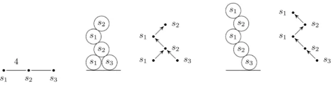
Running Example 1. Consider the finite Coxeter group

W B

( )

2 , whose Coxeter

graph is shown in Figure 3 on the left1_{. In this Coxeter group,}

1 2 1 2 2 1 2 1

s s s s =s s s s , and so the element w=s s s s s3 1 2 1 2 can also be written as w=s s s s s3 2 1 2 1. Both of

these reduced words gives rise to a heap, which are shown in Figure 3. It is easy to see that these two heaps describe different words in the trace monoid *

S , where

{

1

, ,

2 3

}

S

=

s s s

. However, they represent the same group element in

W B

( )

₂ .

Heaps generally do not provide a “magic bullet” for proving theorems in Cox-eter theory or elsewhere, but they are often quite useful. They have been applied to a variety of topics in pure and applied mathematics, physics, computer science,

1_{Normally, the vertices of} _{( )} 2

B

Γ are s s s0, ,1 2, but we are using s s s1, ,2 3, for consistency with the

(4)

[image:4.595.210.541.70.156.2]

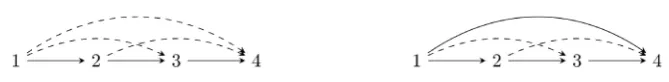
DOI: 10.4236/ojdm.2019.94010 113 Open Journal of Discrete Mathematics Figure 3. The element w=s s s s s3 1 2 1 2=s s s s s3 2 1 2 1 in the Coxeter group W B

( )

2 has two heaps, one for each commutativity class.

and engineering. Examples include fully commutative [4] [5] and freely braided

[6] elements in Coxeter groups, Kazhdan-Lusztig polynomials [7], representa-tions of Kac-Moody [8] and Lie algebras [9], Q-system cluster algebras [10], pa-rallelogram polyominoes [11], q-analogues of Bessel functions [12], Lyndon

words [13], lattice animals [14], Motzkin path models for polymers [15], Lorent-zian quantum gravity [16], modeling with Petri nets [17], control theory of dis-crete-event systems [18], and many more.

Returning to Coxeter groups, heaps provide a framework for reducibility:

commutativity classes of elements correspond to heaps, and reduced words to labeled linear extensions. The goal of this paper is to develop and study a cyclic version of a heap. This was originally motivated by a need for a framework of

cyclic reducibility in Coxeter groups, though we expect that this structure will appear in other settings in combinatorics and beyond. Cyclic reducibility in Coxeter groups is closely related to the conjugacy problem, but it is also inter-esting in its own right. To motivate this connection, note that conjugating a re-duced word

s

i1



s

ik by the initial generator 1 1

1

i i

s =s− cyclically shifts it, e.g.

(

)

1 1 2 k 1 2 k 1. i i i i i i i i

s s s s s =s s s (1.1)

Loosely speaking, one can think of our cyclic version of a heap as the result of identifying (or gluing) the top with the bottom of the diagrams in Figures 1-3, so that the “heap of pieces” is not a vertical stack, but rather a cylinder. For simple examples, such as the ones already given, this concept is visually clear. However, it is much less clear to how to formalize this mathematically and what the un-derlying structure should be, especially for general dependency graphs.

The answer to this involves a fairly new concept of a toric poset, introduced by Develin, Macauley, and Reiner in 2016 [19]. A toric poset is a cyclic version of an ordinary poset, that is generated by the equivalence under making minimal elements maximal, in the sense of Equation (1.1) above. Many fundamental fea-tures of posets have very natural cyclic, or “toric” analogues. For example, a chain in a poset is a totally ordered set, but a toric chain in a toric poset represents a totally cyclically ordered set. An extension of a poset is defined by adding relations. The toric counterpart to this concept is called a toric extension, but in order to see how these are analogous, one has to view things geometrically, and that is where the “toric” name comes from. A finite poset P can be viewed

(5)

chamber

c P

( )

of a graphic hyperplane arrangement



( )

G

in



n_{. Though}

G and hence



( )

G

are not uniquely determined by the poset, the particular

chamber

( )

n

c P ⊆ is. The geometric interpretation of the equivalence

gener-ated by making minimal elements maximal is quotienting out by the integer

lat-tice



n_{. The result is a (toric) hyperplane arrangement}

( )

tor

G



in the n-torus

/

n n

  . The chambers of



tor

( )

G

are in bijection with the acyclic orientations

of G under the equivalence of converting sources into sinks, and these are

called toric posets over G. Now, back to extensions: an extension of a poset can

be described geometrically as adding hyperplanes to the arrangement



( )

G

,

and a (toric) extension of a toric poset corresponds to adding (toric) hyperplanes to



tor

( )

G

. There are also natural toric analogues of linear extensions,

transi-tivity, Hasse diagrams, intervals, antichains, order ideals, morphisms, and P

-partitions, among others. The ones relevant to toric heaps will be discussed later when we formalize them in Section 6. More details about these and others can be found in [19] [20] [21].

The formal definition of a toric poset can be found in Definition/Theorem 5.1. However, now that we have conveyed the intuitive idea of it, we can give the formal definition of a toric heap. It should be thought of as a labeled toric po-set—a cyclic version of an ordinary heap.

Definition 1.3. A toric heap is a triple

(

T

, ,

Γ

τ

)

consisting of a toric poset

T, a graph Γ, and a function τ:T → Γ to its vertex set, satisfying:

1) For every vertex s of Γ, the subset τ−1

( )

{ }

_s is a toric chain in _T,

called a toric vertex chain.

2) For every edge

{ }

s t

,

of Γ_{, the subset} 1

(

{ }

)

,

s t

τ− _{is a toric chain in}_T_,

called a toric edge chain.

3) If T′ is another toric poset over the same set satisfying (1) and (2), then T′ is a toric extension of T.

(6)

commut-DOI: 10.4236/ojdm.2019.94010 115 Open Journal of Discrete Mathematics ative (TFC) and faux CFC. The former are the elements that have only one cyclic commutativity class, and the latter are those that additionally admit long braid relations. Finally, in Section 8, we discuss recent work on reducibility, cyclic re-ducibility, and conjugacy using the toric heap framework. A few beautiful results by T. Marquis in [22] are inaccurate as stated, but easily corrected by replacing “cyclically reduced” with “torically reduced”. We conclude in Section 9 with some open problems and directions for future research.

2. Combinatorial Coxeter Theory

Though the theory of heaps can be developed independently, Coxeter groups provide a wealth of useful and motivating examples, and so we will introduce them right away. More information can be found in classic texts such as Humphreys [23] or Björner and Brenti [24]. In this section, we will begin by de-fining posets over graphs, and then show how they arise in Coxeter theory. That will naturally lead us into heaps, which will be done in Section 3.

2.1. Posets over Graphs

Throughout this paper,

G

=

(

V E

,

)

will be an undirected graph without loops,

P a nonempty finite set, and ≤P a binary relation that is reflexive, antisymmetric, and transitive. The pair

(

P

,

≤

_P

)

is a partially ordered set, or poset. Usually we

will write P instead of

(

P

,

≤

P

)

, as the relation is generally understood.

An acyclic orientation

ω

of G determines a partial ordering on V , where

P

i≤ j if and only if there is an

ω

-directed path from i to j. We denote this

poset by

P

=

P G

(

,

ω

)

, and say that it is a poset on G. Let

Acyc

( )

G

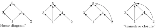
be the set

of all acyclic orientations of G. It should be noted that a (finite) poset does not

uniquely determine a graph. However, given a poset P, there is a unique

mi-nimal graph _ˆHasse

( )

G P with respect to edge-inclusion, called the Hasse

dia-gram, and a unique maximal graph

G P

( )

, called the transitive closure, from

[image:6.595.222.530.650.706.2]

which P arises as an acyclic orientation. A simple example of this is shown in

Figure 4, where acyclic orientations of four different graphs (the undirected ver-sions of those shown) all describe the same 5-element poset.

If for every x≠ y in P, either x≤P y or y≤P x holds, then ≤P is a

total order, and

(

P

,

≤

_P

)

is a totally ordered set. Naturally, we write x<_P y if

P

x≤ y and x≠ y. A totally ordered subset of a poset is called a chain.

2.2. Coxeter Groups

A rank-n Coxeter system is a pair

(

W S

,

)

consisting of a set

S

=

{

s

₁

,



,

s

_n

}

that generates a Coxeter group W by the presentation

(7)

( )

,

1, , | 1 .

i j m

n i j

W = s  s s s =

Each bond strength mi j, :=m s s

(

i, j

)

=1 if and only if si =sj, and mi j, is

precisely the order2_of

i j

s s . Distinct generators s s_i, _j commute if and only if

(

i, j

)

2

m s s = . A Coxeter system has a Coxeter graph Γ which has vertex set

{

1,



,

n

}

(or alternatively,

{

s

₁

,



,

s

_n

}

) and an edge

{ }

i j

,

with label m s s

(

_i, _j

)

for each noncommuting pair of generators. Labels of 3 are usually omitted be-cause they are the most common. A Coxeter system

(

W S

,

)

is irreducible if Γ is connected.

If a word 1

*

w

m

x x

s s S

=  ∈ is equal to w when considered as an element

of W , we say that it is a word or expression for w. If furthermore, m is minimal, we call it a reduced word for w, and we call m its length, denoted



( )

w

. Let

( )

w



be the set of reduced words for w∈W and

(

*

)

,

W S

 be the set of all

reduced words. We typically write words using an upright font, though it is

common to speak of a word *

w∈S as also being a group element w∈W.

For each integer m≥2 and distinct generators s t, ∈S, define

*

, _m .

m s t =stst_{}∈S

A relation of the form , _{( )}_, , _{( )}_,

m s t m s t

s t = t s is a braid relation, and a short braid

relation3_if

_{m s t}

( )

_,

₌

₂

_{. The braid relations generate an equivalence on} *

S , de-noted ≈_{. A classic theorem of Matsumoto}_[25]_{says that the resulting}

equiva-lence classes are in bijection with the elements of W.

Theorem 2.1 (Matsumoto). Any two reduced words for w∈W differ only

by braid relations.

By Matsumoto’s theorem, it is well-defined to let the support of an element

w∈W, denoted

supp

( )

w

, be the set of all generators appearing in any reduced

word for w. If

supp

( )

w

=

S

, then we say that w has full support.

The short braid relations generate an equivalence relation ~ on *

S that is

coarser than ≈_{. The resulting equivalence classes are called}_{commutativity}

classes. Clearly, the reduced words of any w∈W are a disjoint union of

com-mutativity classes, i.e.

( )

w

=

( )

w

1



( )

w

k





for some reduced words w ,1, wk, and where



( )

w

i is the commutativity class that contains wi.

Definition 2.2. An element w∈W is fully commutative (FC) if



( )

w

contains only one commutativity class. Let

FC

(

W S

,

)

denote the set of fully

commutative elements of W .

The classification of finite and affine Coxeter groups is well known, and it consists of several infinite families and some exceptional cases [24]. We will de-note these groups by e.g.

W A

( )

n , W B

( )

n , and their Coxeter graphs by, e.g. 2_{For ease of notation, we allow}

,

i j

m = ∞, and say that w∞: 1= for any w∈W. 3_{Some authors call}

( ), ( ),

, _{m s t} , _{m s t}

s t = t s a short braid relation if m s t

( )

, =3, and a commutation

(8)

( )

A

n

Γ

, Γ

( )

Bn , etc.

Running Example 1 (continued). Consider the word w=s s s s s3 1 2 1 2 as an

element of three different Coxeter groups, one for each of the Coxeter graphs shown below. Recall that we are deliberately using

{

s s s

1

, ,

2 3

}

instead of the

usual

{

s s s

0

, ,

1 2

}

as the generating set of

W B

( )

2 so that all three Coxeter

graphs have the same vertex sets.

The word w=s s s s s3 1 2 1 2 is not reduced in

W A

( )

3 because

(

)

(

)

3 1 2 1 2 3 2 1 2 2 3 2 1

s s s s s

=

s s s s s

=

s s s

. It is reduced in

W B

( )

₂ but not FC,

be-cause

w

=

s s s s s

3

(

1 2 1 2

)

=

s s s s s

3

(

2 1 2 1

)

. The partition of the reduced words into

commutativity classes is

( ) {

w

=

s s s s s

3 1 2 1 2

, .

s s s s s

1 3 2 1 2

} {



s s s s s

3 2 1 2 1

}



Finally, the word w is reduced in

W H

( )

₃ and the corresponding group

ele-ment w has a unique commutativity class,



( ) {

w

=

s s s s s s s s s s

3 1 2 1 2

,

1 3 2 1 2

}

, so it

is FC.

3. Labeled Posets and Heaps

Recall from Definition 1.2 that a heap is a triple

(

P

, ,

Γ

φ

)

, where

φ

:

P

→ Γ

is

a map from a poset to a graph. We will call P the heap poset, Γ the heap

graph, and

φ

the labeling map. Recall that the partial order on P is minimal

(coarsest) such that the preimage 1

( )

s

φ

− _{of each vertex and the preimage}

(

)

1

{ , }s t

φ

− _{of each edge in}_Γ_{are chains. However, when defining the heap}

from a concrete object, such as a reduced word in a Coxeter group, it is also ne-cessary to specify the relative order of the elements within each of these chains. We will do this with an acyclic orientation.

Definition 3.1. Given a word

w

=

s

x1



s

xm in

*

S , consider the graph

(

)

w

,

G

=

V E

, where

V

=

[ ]

m

and E is the set of all

{ }

i j

,

for which

i

≠

j

and

(

,

)

2

i j

x x

m s s ≠ . Let ω_w be the orientation where each edge

{ }

i j

,

is oriented as

i

→

j

if

i

<

j

and

j

→

i

otherwise. Define the poset

P

_w

=

P G

(

_w

,

ω

_w

)

.

Definition 3.2. Fix a Coxeter system

(

W S

,

)

, and let

1

w

m

x x

s

=

_

_{be a}

word in *

S . Define the labeling map

( )

w:Pw , w i sxi.

φ → Γ φ =

The triple



( ) (

w :

=

P

w

, ,

Γ

φ

w

)

is called the heap of w. If

w

∈



( )

w

, then we

say it is a heap of the group element w∈W.

By construction, distinct words in *

S give rise to distinct heaps, even if they are in the same commutativity class. For example, consider the words w=s s s1 3 2

and w′ =s s s3 1 2 in

W A

( )

3 . Even though w ~ w′, the heaps



( )

w

and

( )

w

′



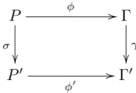
are different. We would like to say that they are “the same,” and we can

do this using the concept of a heap isomorphism from [3]. Let Heap be the cat-egory of heaps, where morphisms are defined below.

(9)

is a pair

( )

σ γ

,

, where σ:P→P′ is a poset morphism and γ :Γ → Γ′ is a

graph homomorphism, satisfying γ φ φ σ_ = ′_ _:

If

( )

σ γ

,

is a heap morphism with γ being the identity map on Γ = Γ′,

and

σ

is injective, then

(

P

′ ′ ′

,

Γ

,

φ

)

is a subheap of

(

P

, ,

Γ

φ

)

. If

σ

and γ

are both bijective, then the two heaps are isomorphic. If we want to only consid-er heaps ovconsid-er a fixed graph Γ_{, which is often the case, we can define}

Heap

( )

Γ

.

We will mostly refrain from the category theory point of view in this paper, be-cause the focus is more on Coxeter theory. A thorough categorical treatment of heaps and toric heaps will be done in a forthcoming paper. However, in order to

speak about morphisms in Coxeter theory where Γ ≠ Γ′, we would need to be

clear on how to define a homomorphism between Coxeter graphs, especially re-garding edge weights. We will not do that here because we will not be using it.

Proposition 3.4. If w ~ w′ are reduced words in

(

W S

,

)

, then the heaps

( )

w



and



( )

w

′

are isomorphic.

Proof. Since w and w′ differ by a sequence of short braid relations, it

suf-fices to consider the case when they differ by a single adjacent transposition

1 1

i i i i

x x x x

s s

s

+

↔

+ . In this case, the heap isomorphism is

( )

σ γ

,

, where the

trans-position

σ =

(

i i

+

1 )

is a poset isomorphism and γ is the identity. _

Henceforth, we will always speak of heaps up to isomorphism. By Proposition 3.4, each commutativity class of w has a unique heap. Therefore, if w is FC, then we may speak of



( )

w

:

=



( )

w

as the heap of the group element w. In contrast, for non-FC elements, different commutativity classes generally give non-isomorphic heaps. Our running example illustrates this nicely.

Running Example 1 (continued). Let us recall w=s s s s s3 1 2 1 2 first as an

element in the Coxeter group

W B

( )

2 , and then in

W H

( )

3 . In

W B

( )

2 , it has

two commutativity classes, and the associated heaps were shown in Figure 3. In

( )

3

W H

, the bond strength between s₁ and s2 is increased to

m s s

(

1

,

2

)

=

5

.

This means that w=s s s s s3 1 2 1 2 is FC, and so the only heap of this group

ele-ment is the first one shown in Figure 3.

Heaps of reduced words in Coxeter groups were studied by Stembridge in [4], though his definition was slightly different, in that he considered i and j

incomparable if sxi =sxj. For reduced words, this makes no difference. In our

setting, such an i and j must be comparable because the φ-preimage of

[image:9.595.325.424.105.173.2]

(10)

The concept of a labeled linear extension of a heap was studied in [4]. Here, we give an abstract definition of a more general concept in our framework. We also drop the word “labeled” because it is implied in the context of heaps. Say that a map γ :Γ → Γ′ is an edge-inclusion if it is the identity map between

graphs on the same vertex set, and every edge in Γ_{is also in} Γ′.

Definition 3.5. If

(

P

′ ′ ′

,

Γ

,

φ

)

is the image of a morphism from a heap

(

P

, ,

Γ

φ

)

, where σ:P→P′ is an extension, and γ :Γ → Γ′ is an

edge-inclusion, then we say that it is an extension of

(

P

, ,

Γ

φ

)

. Moreover, it is a linear extension of heaps if

σ

is a linear extension of posets.

Given a heap

(

P

, ,

Γ

φ

)

and a graph homomorphism γ :Γ → Γ′, there need

not be a poset P′ and a map σ:P→P′ such that

( )

σ γ

,

is a morphism to a

heap

(

P

′ ′ ′

,

Γ

,

φ

)

. However, there will always be (at least) one if γ is an

edge-inclusion, and it is easy to see how to construct P′—it is a poset generated

by the relations in P with edge chains for each additional edge in Γ′. In

gen-eral, such a P′ is not unique because there could be a choice of how to order

the elements within each new edge chain, as shown in the following simple ex-ample.

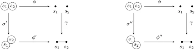
Example 3.6. Let γ :Γ → Γ′ be the edge-inclusion between the edgeless

graph on

V

=

{

v v

1

,

2

}

to the complete graph. The antichain

P

=

{ }

1, 2

and

labeling map

φ

( )

i

=

v

i define a heap

(

P

, ,

Γ

φ

)

. There are two linear extensions of P: let P′ denote the one with 1<P′ 2 and P′′ the one with 2<P′′1. There are canonical heap morphisms

(

σ γ

′

,

)

and

(

σ γ

′′

,

)

from

(

P

, ,

Γ

φ

)

to

(

P

′ ′ ′

,

Γ

,

φ

)

and

(

P

′′ ′ ′′

, ,

Γ

φ

)

, respectively. Here, σ′ and σ′′ both send ii,

and φ′_and φ′′_{both send} iv_i. These are shown in Figure 5.

Let

 

( )

denote the set of linear extensions of a heap . In [4], these are

called labeled linear extensions because they can be canonically indexed by

words. For example, a linear extension

(

P

′ ′ ′

,

Γ

,

φ

)

can be described by the

word

φ

′

( )

x

1



φ

′

( )

x

m , where x1<P′<P′ xm.

Example 3.7. Let

(

P

, ,

Γ

φ

)

be the heap from Figure 1 and

(

P

′ ′ ′

,

Γ

,

φ

)

the

heap from Figure 2. Note that it is easy to define the labeling maps

φ

and φ′

to adapt those heaps to our framework. Since σ:P→P′ is an extension and γ an edge-inclusion, the morphism

( )

σ γ

,

is an extension of heaps. The total

order w=acbabgdfe uniquely describes a heap that is a linear extension of

both

(

P

, ,

Γ

φ

)

and

(

P

′ ′ ′

,

Γ

,

φ

)

.

[image:10.595.214.538.620.707.2]

In the examples from Figure 5, the two linear extensions are clearly characte-rized by the words w′ =s s1 2 (left) and w′′ =s s2 1 (right).

(11)

4. Coxeter, FC, and CFC Elements

One of the goals of this paper is to develop a framework for studying what we call “cyclic reducibility” in Coxeter groups. In this section, we will formalize concepts such as cyclic words and cyclic commutativity classes. In a subsequent section, we will develop a cyclic version of a heap called a toric heap, which is essentially a labeled toric poset. To motivate this, we will begin with conjugation of Coxeter elements, and then extend that to the cyclically fully commutative (CFC) elements. Throughout, let

(

W S

,

)

be a fixed Coxeter system with

Cox-eter graph Γ_{. Given words, e.g.}

c, w, w

′

in *

S , we will denote the

corres-ponding group elements by

c w w

, ,

′

in W.

4.1. Conjugation of Coxeter Elements

Let

(

W S

,

)

be a Coxeter system. A Coxeter element is the product of all

gene-rators in some order. We denote the set of all Coxeter elements by

C

(

W S

,

)

.

Every Coxeter element of

(

W S

,

)

gives rise to a canonical acyclic orientation of

the Coxeter graph Γ_{, defined by}

( )

(

)

₁

: Acyc C , , : ,

n

x x

c Γ → W S c ω s s

where

s

x1



s

xn is any linear extension of

P

(

Γ

,

ω

)

. It is easy to see that this

map is a bijection, and so we write

c

( )

ω

to denote “the Coxeter element

de-fined by

ω

_{”, and}

ω

( )

c

for “the acyclic orientation given by c”. Since Cox-eter elements are FC, the heap poset of

c

∈

C

(

W S

,

)

does not depend on the

choice of reduced word, so we may write Pc:=Pc.

Proposition 4.1. The heap poset of a Coxeter element c is P_c=P

(

Γ,ω

( )

c

)

for any reduced word c.

Proof. Let

c

=

s

x1



s

xn. By construction,

P

c

=

[ ]

n

, and the labeling map

c:Pc

φ → Γ_{is defined by}

φ

c

( )

i =sx_i . Since c has no repeated generators,

each preimage 1

( )

i

x

s

φ− _{has size 1, and so is trivially a chain. For each edge}

{

,

}

i j

x x

s s in Γ, say

i

<

j

without loss of generality, the preimage

{

}

(

)

{ }

1

, ,

i j

x x

s s i j

φ− ₌ _{is a chain with}

c

P

i

<

j

. This matches the orientation of

the edge

{ }

i j

,

by

ω

( )

c

from Definition 3.1. _

Since linear extensions of heaps can be indexed with words, we can consider the set  

(

( )

w

)

as a collection of words in S*. A subset of S* is said to be

order-theoretic if it is the set of linear extensions of a heap. The following is a slight reformulation of Theorem 3.2 from [4].

Proposition 4.2.For an element w∈W, the following are equivalent:

1) w is fully commutative. 2)



( )

w

is order-theoretic.

3) 

( )

w = 

(

( )

u

)

for some (equivalently, every)

u

∈



( )

w

.

(12)

Coxeter element is also a Coxeter element, and because 1

s=s− for every s∈S,

it is also a conjugation by the initial letter:

(

)

1 1 2 m 1 2 m 1. x x x x x x x x

s s s s s =s s s

On the level of acyclic orientations, these two Coxeter elements are related by converting the source vertex

s

x1 (an initial generator) into a sink (a terminal

generator). This generates an equivalence relation ≡_on

Acyc

( )

Γ

, and hence

on

C

(

W S

,

)

, that we call toric equivalence. This was first studied by Pretzel in [26] via an operation he called “pushing down maximal vertices”. In [27], H. Eriksson and K. Eriksson showed that these equivalence classes are in 1-1 cor-respondence with the conjugacy classes of

C

(

W S

,

)

. In a recent preprint of

Adin et al. that introduces toric P-partitions, these equivalence classes are

called toricDAGs [21].

Theorem 4.3 ([27]). In any Coxeter group,

c c

,

′∈

C

(

W S

,

)

are conjugate if

and only if

ω

( )

c

≡

ω ′

( )

c

.

Thus, there are bijections between the Coxeter elements and

Acyc

( )

Γ

, and

between their conjugacy classes and toric equivalence classes, defined as follows:

(

)

( )

(

)

( )

C , Acyc Conj C , Acyc /

cl_W

W S W S

c ω c c ω c

→ Γ → Γ ≡

 

 

 

The sets

Acyc

( )

Γ

and

Acyc

( )

Γ ≡

/

are enumerated by the Tutte polynomial

( )

,

T

_Γ

x y

at

( ) ( )

x y

,

=

2, 0

and

( ) ( )

x y

,

=

1, 0

, respectively [19].

Example 4.4.Consider the affine Coxeter group W=W A

( )

3 , whose Coxeter

graph is the circular graph C4. Consider the following three reduced words for

Coxeter elements: c1=s s s s1 2 3 4, c2=s s s s1 3 2 4, and c3=s s s s1 4 3 2 (using s4

in-stead of the usual s0). The corresponding acyclic orientations are shown below

4_.

(4.1)

The 4!=24 reduced words for Coxeter elements in W A

( )

₃ comprise

( )

4

Acyc C =2 − =2 14 distinct elements. The 14 acyclic orientations fall into

( )

4

Acyc C /≡ =3 toric equivalence classes: ω

( )

c1  and ω

( )

c3  have size

4, and ω

( )

c2  has size 6, the elements of which are shown below.

(4.2)

By Theorem 4.3, the 14 Coxeter elements fall into 3 distinct conjugacy classes, and any two conjugate Coxeter elements differ only by cyclic shifts and short braid relations. This can be visualized by writing the reduced words as circular words, and allowing the usual braid relations:

(13)

applied, so both c1 and c3 are conjugate to only 4 Coxeter elements each—all

cyclic shifts. In contrast, the relations s s1 3=s s3 1 and s s2 4 =s s4 2 can be

ap-plied to

[ ]

c

2 , yielding three other “reduced cyclic words”:

(4.3)

There are six distinct Coxeter elements, and 16 reduced words, that can arise from these four cyclic words, assuming they are read off clockwise:

1 2 4 3 2 4 1 3 4 1 3 2 2 1 3 4 1 3 2 4 3 2 4 1

1 4 2 3 2 4 3 1 4 3 1 2 2 3 1 4 1 3 4 2 3 4 2 1

4 2 3 1 3 1 4 2

4 2 1 3 3 1 2 4

s s s s s s s s s s s s s s s s s s s s s s s s

s s s s s s s s

= = = = = =

= =

(4.4)

The elements in the ith_{column above are the linear extensions of the poset} de-fined by the ith_{orientation in Equation (4.2).}

Example 4.4 should motivate the value of developing a theory of cyclic redu-cibility in Coxeter groups. For example, the four cyclic words in Equation (4.3) should be thought of as lying in the “cyclic commutativity class” containing the “cyclic word”

[ ]

c

2 . In Section 6, we will develop this framework. But first, we

need to focus on the curious “cyclic partial order” structure that arises. Cyclic words under the equivalence generated by short braid relations are like cyclic analogues of traces, though without the monoid structure, because there is no canonical way to concatenate cyclic words. This cyclic poset structure can be formalized via toric posets [19], which leads to the concept of a toric heap. This is essentially a labeled toric poset, in the same sense of how ordinary heaps are labeled ordinary posets. It allows us to extend the examples shown in this section far beyond just Coxeter elements, which we will do next.

4.2. Cyclically Fully Commutative (CFC) Elements

Now that we have seen the interplay between Coxeter elements, acyclic orienta-tions, and heaps, and how they behave under conjugacy, we will extend these ideas to a larger class of elements. This will elucidate the key structural proper-ties as well as motivate the main ideas of our cyclic reducibility framework.

It is well known that in any Coxeter group, if s∈S, then



( ) ( )

sw

=



w

±

1

,

and so _

( )

_wk ≤_k_

( )

_w . If equality holds for all _k_∈, then we say that _w is logarithmic5_{. In 2009, it was shown independently by D. Speyer}_[28]_{and H.} Eriksson and K. Eriksson [27] that in infinite irreducible Coxeter systems, Cox-eter elements are logarithmic. It is simple to extend this to the non-irreducible

(14)

case—each connected component of Γ must be the Coxeter graph of an

infi-nite group. The logarithmic property was key to the Erikssons’ proof of the con-jugacy problem (Theorem 4.3). Also crucial was the source-to-sink property, i.e.

toric equivalence. In plain English, we mean that 1) Coxeter elements are FC (they avoid long braids), and 2) cyclic shifts of Coxeter elements remain FC. These properties can naturally be extended beyond Coxeter elements.

Definition 4.5. An element w∈W is cyclically fully commutative (CFC) if

for any reduced word of w, every cyclic shift is reduced and FC.

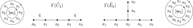
Example 4.6. Figure 6 shows examples of CFC elements in two affine Coxeter

groups. On the left is the Coxeter graph of the group W C

( )

4 and the CFC

ele-ment w1=s s s s s s s s0 1 2 3 4 3 2 1 drawn in a circle so the reader can visually see how

there are no long braids. To the right is the Coxeter graph of the group W E

( )

6

and the CFC element w2 =s s s s s s s s s s s s1 3 2 4 3 5 4 6 0 3 2 6, also drawn in a circle.

CFC elements were introduced and studied in 2012 by Boothby et al. [29].

They have recently been characterized and enumerated in all affine Coxeter groups, and their generating functions were shown to be rational in all Coxeter groups [30] [31].

5. Labeled Toric Posets and Toric Heaps

5.1. Posets and Toric Posets, Geometrically

Throughout this section, Γ is a Coxeter graph,

G

=

(

V E

,

)

is an undirected

graph,

Acyc

( )

G

is the set of acyclic orientations of G, and ≡ is toric

equi-valence, i.e. the equivalence relation on

Acyc

( )

G

generated by source-to-sink

conversions.

A toric poset should be thought of as a cyclic version of a poset. The most concrete way to define them are as toric equivalence classes of

Acyc

( )

G

, and

we write this as, e.g. T G

(

,

[ ]

ω

)

. However, this has two significant drawbacks:

first, it suggests a dependence on the graph G, which is a little misleading. Recall

that we can similarly define a poset

P

=

P G

(

,

ω

)

on a graph, though in actuality,

G is almost never uniquely determined. Specifically, there is a unique minimal

graph (the Hasse diagram, _ˆHasse

( )

G P ), and a unique maximal graph (the

transi-tive closure,

G P

( )

) on V such that any

G

′

=

(

V E

,

′

)

whose edge set E′ is

between the edge sets of these two extremes (with respect to subset inclusion) will work. Of course, care must also be taken with how to define

ω′

∈

Acyc

( )

G

′

so that

P G

(

,

ω

)

=

P G

(

′ ′

,

ω

)

, but that is straightforward—any shared edges

[image:14.595.212.537.636.683.2]

must be oriented the same way.

(15)

The second drawback of the notation T G

(

,

[ ]

ω

)

is that it obscures the “more

proper” geometric way to define a toric poset. We will motivate this by revisiting the geometric interpretation of

P G

(

,

ω

)

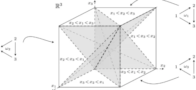
. In fact, finite posets can be defined

and developed purely geometrically, as chambers of graphic hyperplane arrange-ments. For distinct vertices i and j in V, let H_ij be the hyperplane x_i =x_j

in



V_{. The graphic arrangement of}

G is the set 

( )

G =

{

H_ij|

{ }

i j, ∈E

}

. Each

point

x

=

(

x

1

,



,

x

n

)

in the complement

( )

V G

−

  determines a canonical

acyclic orientation

ω

( )

x

, by directing the edge

{ }

i j

,

as

i

→

j

if x_i <x_j.

The fibers of this mapping are the chambers of the



( )

G

, and so this induces a

bijection between chambers of



( )

G

and acyclic orientations of G:

At this point, one could define a poset to be any subset of



V_{that arises as a} chamber of some graphic hyperplane arrangement. This removes the reference to a particular graph in the definition. Given a poset P, we write

c P

( )

for the

chamber in



V_{determined by}

P. Given a chamber c, we write

P c

( )

for

the poset determined by c.

Though this geometric perspective is a bit superfluous for ordinary posets, it is absolutely necessary for toric posets, where it is not so clear how to pull apart the concept of a toric poset from the underlying graph. The geometric definition of a toric poset arises from the observation that if we first quotient out



V_{by the} integer lattice



V_{, then converting a source}

i

x into a sink corresponds to

crossing a coordinate hyperplane xi =0, and this does not change the

corres-ponding connected component in the torus  V / V. An example of this is

shown in Figure 7.

[image:15.595.217.535.514.660.2]

This leads us to our first of five “Definition/Theorems”. We use that term

Figure 7. The hyperplane arrangement 

( )

G of the complete graph G=K3. The

tor-ic arrangement tor

( )

G is achieved by identifying opposite sides of the unit cube. Doing

(16)

because each of them involves a non-trivial statement or equivalence proven in

[19], which allows us to take them as the definition in this paper.

Definition/Theorem 5.1. A toric poset over G is characterized by either:

1) an equivalence class

[ ]

ω

in

Acyc

( )

G

/

≡

,

2) a chamber c of the toric hyperplane arrangement



tor

( )

G

in /

V V

  .

We will write T G

(

,

[ ]

ω

)

to mean the toric poset characterized by

[ ]

ω

in

( )

Acyc

G

/

≡

. Given a toric poset T, we write

c T

( )

when we wish to speak of

the chamber in  V / V determined by T, and given a chamber c, we write

( )

T c

to emphasize the toric poset determined by it.

Aside from the definition not depending on a distinguished graph G, the

second advantage to the geometric perspective is the recurring theme that many standard features of ordinary posets, such as chains, antichains, Hasse diagrams, transitive closure, order ideals, and so on, have natural toric analogues. However, it is usually not clear how these should be defined in terms of an equivalence class of acyclic orientations. Instead, the natural definition often only becomes apparent when one interprets the classical definition geometrically, and then passes to the quotient π:V → V / V , as illustrated by the following com-mutative diagram:

Often, this toric analogue then has a natural combinatorial interpretation in terms of directed graphs, which usually ends up being more convenient. A list of these can be found in the Introduction of [20].

For an example of this, consider a non-edge

{ }

i j

,

∉

E

. One might ask

whether i and j are comparable in

P

=

P G

(

,

ω

)

. In other words, would

add-ing

{ }

i j

,

to G force its orientation by

ω

, which happens when one of the

two ways to orient it would create a directed cycle? If so,

{ }

i j

,

is implied by tran-sitivity, and either i≤P j or j≤P i. Geometrically, this means that the hyper-plane Hij is disjoint from the chamber

c P

( )

of



( )

G

. The combinatorial

condition is also straightforward:

{ }

i j

,

is implied by transitivity if and only if

i and j lie on a common directed path in

ω

(i.e. lie on a chain in P).

There is a toric analogue of transitivity, which is easy to state geometrically: the edge

{ }

i j

,

is implied by toric transitivity if the toric hyperplane tor

ij

H is

disjoint from the chamber c T G

(

,

[ ]

ω

)

of



tor

( )

G

. The combinatorial

con-dition of this is less clear due to the absence of a binary relation, but luckily, it has a simple answer, which is basically just adding the word “toric” to the ordinary case. Specifically, a toric directed path in

ω

_{is a directed path}i₁→→i_k such that the edge i1→ik is also present, as shown in Figure 8. It was shown in [19] that if i1→→ik is a toric directed path in

ω

, then some cyclic shift is a toric directed path in ω′_{for each}ω′ ≡ω_.

(17)

DOI: 10.4236/ojdm.2019.94010 126 Open Journal of Discrete Mathematics Figure 8. A chain in a poset is any subset that lies on a directed path (left). A toric chain in a toric poset is any subset that lies on a toric directed path (right).

toric directed path is an edge, and all vertices are one-element toric directed paths. We will say that the empty set is vacuously a directed path and a toric di-rected path.

Definition/Theorem 5.2. A non-edge

{ }

i j

,

is implied by transitivity in

(

,

)

P G

ω

if and only if i and j lie on a directed path in

ω

.

A non-edge

{ }

i j

,

is implied by toric transitivity in T G

(

,

[ ]

ω

)

if and only if

i and

j

lie on a toric directed path in

ω

.

For ordinary posets, adding all edges implied by transitivity, in any order, yields the transitive closure, G P G

(

,ω

)

. The toric transitive closure

[ ]

(

)

(

)

tor

,

G T G ω can be defined analogously.

For ordinary posets, removing all unnecessary edges, in any order, yields the

Hasse diagram, denoted _ˆHasse

(

)

,

G P G ω . Geometrically, this just means

remov-ing all hyperplanes Hij that are disjoint from the chamber c P G

(

,ω

)

. The toric Hasse diagram is completely analogous, and denoted _ˆtorHasse

(

[ ]

)

,

G T G ω .

However, the Hasse diagram of

P G

(

,

ω

)

and the toric Hasse diagram of

[ ]

(

,

)

T G ω are generally not the same. To see why, we need the notion of a toric

chain.

A key concept behind the aforementioned features of posets is that of a chain, which is a totally ordered set. This can be characterized geometrically in terms of the coordinates of the entries of all points in the corresponding chamber, or combinatorially as a subset of vertices lying on a directed path in

ω

. A toric chain in T G

(

,

[ ]

ω

)

is a totally cyclically ordered set. This can also be

characte-rized geometrically in terms of the coordinates of the entries of all points in the corresponding toric chambers. Luckily, its combinatorial characterization is both simple and analogous to the ordinary poset case.

Definition/Theorem 5.3. A set

C

=

{

i

1

,



,

i

k

}

⊆

V

is a:

• chain of

P G

(

,

ω

)

if it lies on a directed path in

ω

;

• toric chain of T G

(

,

[ ]

ω

)

if it lies on a toric directed path in

ω

.

Both chains and toric chains are closed under subsets.

Example 5.4. Let L4, C4, and K4 be the line, circular, and complete graph

on 4 vertices, respectively. Assume that the vertices are ordered “naturally,” i.e.

they all contain (at least) the edges

{ }

1, 2

,

{ }

2,3

, and

{ }

3, 4

. Define

( )

4

Acyc

L

ω ∈

,

ω′∈

Acyc

( )

C

4 , and

ω′′∈

Acyc

( )

K

4 so that

{ }

i j

,

is oriented

i

→

j

if

i

<

j

. Then

(

)

(

)

[ ]

(

)

(

)

(

)

(

)

(

[ ]

)

[ ]

(

)

(

)

tor Hasse

4 4 4

4 4

torHasse tor

4 4 4 4

ˆ _, _, _, _, _,

ˆ _, _, _, _.

G P L K G T C

G P K L

G T K C G T L L

ω ω ω ω ω ′ ′′ = = = ′′ = =

(18)

[image:18.595.205.540.66.107.2]

DOI: 10.4236/ojdm.2019.94010 127 Open Journal of Discrete Mathematics Figure 9. Left: The Hasse diagram of P L

(

4,ω

)

consists of the solid edges (undirected).

The dashed edges are additionally implied by transitivity. Right: The toric Hasse diagram of T K

(

4,

[ ]

ω′′

)

consists of the solid edges (undirected). The dashed edges are implied by

toric transitivity. See Example 5.4 for details.

make up the Hasse and toric Hasse diagram. The transitive closure and toric transitive closure are given by including the (undirected) dashed edges as well.

The last concepts that we need the toric analogue of are extensions and total orders. A total order is a poset

P K

(

_V

,

ω

)

, where K_V is the complete graph. Geometrically, this corresponds to a chamber of



( )

K

V . Intuitively, a total toric order is a toric poset that is totally cyclically ordered.

Definition/Theorem 5.5. A total toric order is characterized by either: 1) a toric poset T K

(

_V,

[ ]

ω

)

,

2) a chamber of



tor

( )

K

V .

An extension P′ of a poset P is characterized combinatorially by adding

relations (or edges to

(

G

,

ω

)

), or geometrically by

c P

( )

′ ⊆

c P

( )

in



V_(the result of adding hyperplanes to



( )

G

). Moreover, P′ is a linear extension of

P if it is an extension and a total order.

Definition/Theorem 5.6. Let T =T G

(

,

[ ]

ω

)

be a toric poset, and assume

without loss of generality that

G

=

(

V E

,

)

is its toric Hasse diagram. A toric extension T′ of a toric poset T is characterized by either:

1)

c T

( )

′ ⊆

c T

( )

in  V / V,

2) T′=T G

(

′,

[ ]

ω′

)

, where

G

′

=

(

V E

,

′

)

,

E

⊆

E

′

, and all edges in

E



E

′

are oriented the same way by

ω

_andω′_.

If T′ is a toric extension of T and a total toric order, then it is a total toric

extension.

There are Acyc

( )

2, 0 !

V

V K

K =T =n total orders on a size-n set V, where

V

K

T

is the Tutte polynomial. In contrast, there are

( )

( ) (

)

Acyc KV /≡ =TK_V 1, 0 = n−1 !

total toric orders on V. Each one is indexed by a cyclic equivalence class of

permutations

[ ]

w

=

[

w

1



w

n

] {

:

=

w w

1 2



w w

n−1 n

,

w

2



w w w

n−1 n 1

,



,

w w w

n 1 2



w

n−1

}

.

Geometrically, these correspond to the

(

n

−

1 !

)

toric chambers of



_tor

( )

K

_V .

5.2. Toric Heaps

Before we formalize cyclic reducibility, it is worth pausing to return to our fa-miliar example for guiding intuition. Recall (see Definition 1.3) that a toric heap has a labeling map τ:T→ Γ such that the inverse image of every vertex and

every edge is a toric chain. Moreover, T must be minimal with respect to these

(19)

Running Example 1 (continued). Recall that the element

3 1 2 1 2 3 2 1 2 1

w=s s s s s =s s s s s in

W B

( )

2 has two distinct heaps, shown in Figure 3.

Note that in each heap, the edge chain φ−1

(

{ }

_{1, 2}

)

forms a length-4 directed

path in the Hasse diagram, and the size-3 edge chain φ−1

(

{ }

_{2, 3}

)

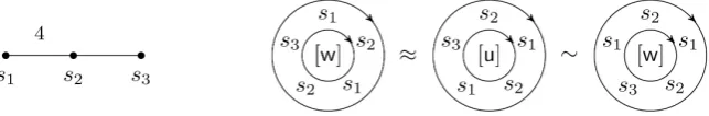
lies on a

length-4 directed path. In the toric heap, these directed paths become toric di-rected paths, and so the toric Hasse diagram gets two additional edges. This is shown in Figure 10; the curved edges are these two additional ones.

Note that the two toric heaps shown in Figure 10 are actually the same, because the Hasse diagrams of the toric heap posets differ by a single source-to-sink conversion. Algebraically, this is because the word s s s s s3 1 2 1 2 can be

trans-formed into s s s s s3 2 1 2 1 two ways: by a long braid relation s s s s1 2 1 2s s s s2 1 2 1, or

by a sequence of short braid relations and cyclic shifts. When we formalize this, we will say that the cyclic words

[ ]

w

=

[

s s s s s

3 1 2 1 2

]

and

[ ]

u

=

[

s s s s s

3 2 1 2 1

]

are in

the same cyclic commutativity class. This is shown in Figure 11.

We can define structure-preserving maps between toric heaps using commut-ative diagrams in the same manner that we did between ordinary heaps in Defi-nition 3.3. This leads to the category torHeap of toric heaps and toric heap morphisms. To properly define a toric heap morphism, we need the definition of a general toric poset morphism. However, we will omit this and instead refer the reader to [20], because in this paper, the only morphisms we will use are exten-sions and isomorphisms. The former has been introduced and the latter is ele-mentary: if there is a graph isomorphism GG′ carrying the acyclic

orienta-tion ω_ω′_{, then the toric posets} T G

(

,

[ ]

ω

)

and T G

(

′,

[ ]

ω′

)

are isomorphic.

[image:19.595.210.543.446.524.2]

Alternatively, it is straightforward to define this geometrically.

Figure 10. Though the element w=s s s s s3 1 2 1 2=s s s s s3 2 1 2 1 in the Coxeter group W B

( )

2 has two distinct heaps (see Figure 3), one for each commutativity class, both of these give rise to the same toric heap. Intuitively, one can think of this as identifying the top with the bottom of a stack of balls, making it cylindrical. The undirected versions of the di-graphs shown are the toric Hasse diagrams of the toric heap posets.

Figure 11. A non-CFC element with only one cyclic commutativity class. The cyclic word

[ ]

u shown in the middle differs from

[ ]

w via a long braid relation s s s s2 1 2 1s s s s1 2 1 2,

but also via a short braid relation, s s1 3s s3 1. This will be formalized in Section 6; this

[image:19.595.214.536.609.662.2]