ISSN Print: 2159-4465
DOI: 10.4236/jsip.2019.103005 Aug. 8, 2019 59 Journal of Signal and Information Processing
Adaptive Lossy Image Compression Based on
Singular Value Decomposition
Marcos Roberto e Souza, Helio Pedrini
Institute of Computing, University of Campinas, Campinas, SP, Brazil
Abstract
Image compression techniques aim to reduce redundant information in order to allow data storage and transmission in an efficient way. In this work, we propose and analyze a lossy image compression method based on the singular value decomposition using an optimal choice of eigenvalues and an adaptive mechanism for block partitioning. Experiments are conducted on several im-ages to demonstrate the effectiveness of the proposed compression method in comparison with the direct application of the singular value decomposition.
Keywords
Image Compression, Adaptive Decomposition, Lossy Compression
1. Introduction
Advances in digital imaging and video acquisition equipments, such as cameras, cell phones, and tablets, have enabled the generation of large volumes of data. Many applications use images and videos, such as medicine [1], remote sensing [2], microscopy [3], surveillance and security [4].
Adjacent pixels in images and videos usually have a high correlation, which leads to redundancy and demands high storage consumption. In order to reduce the space required and the transmission time of images and videos, several com-pression techniques have been proposed in the literature. These techniques ex-plore data redundancies and are generally classified into two categories of com-pression methods: lossless and lossy.
In lossless compression methods, the original data can be completely recov-ered after the decompression process [4], whereas, in lossy compression me-thods, certain less relevant information is discarded, such that the resulting im-age is different from the original imim-age. Ideally, this loss should be tolerated by the receiver [4].
How to cite this paper: e Souza, M.R. and Pedrini, H. (2019) Adaptive Lossy Image Compression Based on Singular Value Decomposition. Journal of Signal and In-formation Processing, 10, 59-72.
https://doi.org/10.4236/jsip.2019.103005
Received: June 16, 2019 Accepted: August 5, 2019 Published: August 8, 2019
Copyright © 2019 by author(s) and Scientific Research Publishing Inc. This work is licensed under the Creative Commons Attribution International License (CC BY 4.0).
http://creativecommons.org/licenses/by/4.0/
DOI: 10.4236/jsip.2019.103005 60 Journal of Signal and Information Processing As the main contribution of this work, we present and evaluate a lossy-based image compression method based on the singular value decomposition (SVD) technique [5] [6]. The originality of the method resides mainly in the choice of eigenvalues and the partitioning of the images in an adaptive way, as well as a detailed investigation in the use of the SVD for the image compression. Experi-ments show that the proposed method is able to achieve better results than those obtained with the direct application of SVD. In addition, new insights to the singular value decomposition-based compression method are provided.
This paper is organized as follows. Some relevant concepts and approaches related to the topic under investigation are briefly described in Section 2. The proposed method for image compression using singular value decomposition is presented in Section 3. The results are reported and discussed in Section 4. Final considerations are presented in Section 5.
2. Related Work
Compression techniques [7]-[16] play an important role in the storage and transmission of image data. Their main purpose is to represent an image in a very compact way, that is, through a small number of bits without losing the es-sential content of the information present in the image.
Image compression methods are generally categorized into lossless and lossy approaches [17] [18] [19]. In lossless compression, all information originally contained in the image is preserved after it is uncompressed. In lossy compres-sion, only part of the original information is preserved when the images is un-compressed.
Image compression methods are based on reducing redundancies in the data representation. The redundancies present in images can be divided into three categories [4] [20]. The coding redundancy refers to the use of a number of bits greater than absolutely necessary to represent the intensities of the pixels of the image. The interpixel redundancy is associated with the relation or similarity of neighboring pixels. Finally, the psychovisual redundancy concerns the imper-ceptible details of the human visual system.
Some lossless compression methods that explore coding redundancy are Huffman coding [21], Shannon-Fano coding [22], arithmetic coding [23] and dictionary-based encoding such as LZ78 and LZW [24]. Run-length coding [25], bit plane coding [26] and predictive coding [27] explore interpixel redundancy. Lossy compression methods, such as predictive coding by delta modulation (DM) [28] [29] or by differential pulse-code modulation (DPCM) [30] and transform coding [31] [32], typically explore psychovisual redundancy.
DOI: 10.4236/jsip.2019.103005 61 Journal of Signal and Information Processing (WDR), in which the input image is first compressed using the SVD and then compressed again with the WDR.
In this work, we apply the use of singular value decomposition in image com-pression and analyze its use locally and with an optimal choice of eigenvalues.
3. Adaptive Image Compression
In this section, we present our adaptive image compression approach based on singular value decomposition, the image partitioning process and the compres-sion evaluation metrics.
3.1. Image Compression
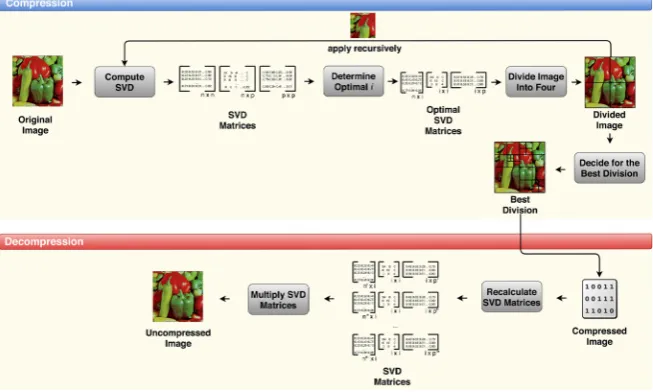
The diagram presented in Figure 1 presents the main steps of the image com-pression and decomcom-pression method proposed in this work. The comcom-pression algorithm has as input an image In p× and, as output, the compressed image represented by the singular value decomposition matrices in a binary file. The decompression algorithm has as input the binary file containing the decomposi-tion matrices and, as output, an image Jn p× ≈In p× . The steps of the method are presented in detail as follows.
Initially, we calculate the singular value decomposition (SVD) for the entire image. The SVD of a real matrix An p× corresponds to the factorization
T
A U V= Σ
where U is a real unit matrix n n× , Σ is a diagonal rectangular matrix n p×
with diagonal nonnegative real numbers and V is a real unit matrix p p× . Since U and VTU are real unitary matrices, then UUT=I and VVT=I,
where I is the identity matrix. Thus, U and VT are orthogonal matrices. The columns of U are the eigenvectors of the matrix AAT, the columns of V are the eigenvectors of the matrix A AT and the diagonal elements of the matrix Σ are the square roots of eigenvalues of AAT or A AT . The eigenvalues are ar-ranged in the matrix Σ in descending order, that is, if σi are the diagonal elements of Σ, then σ1 ≥σ2 ≥≥σn >0. Then,
[
]
T 1 1 T 2 T 2 1 2 TT T T
1 1 1 2 2
0 0 0 0 0 0 n n n n n
A U V
σ σ
σ
σ σ σ
= Σ =
= + 2 + + n
v v
u u u
v
u v u v u v
(1)
Using the entire SVD arrays, with σ1, , σn, would typically make SVD ma-trices larger than the original matrix. Since we are interested in lossy compres-sion, some of the eigenvalues above a certain σi can be discarded, decreasing the final size of the three matrices.
Considering that the σi elements are sorted in descending order, the first
terms T
i i iσ
DOI: 10.4236/jsip.2019.103005 62 Journal of Signal and Information Processing
Figure 1. Main stages of the image compression and decompression process.
(
)( ) ( )( )
opt_value arg max= i
α
−1λ
i +α δ
i (2)where λi is the variance maintained by choosing the first i eigenvalues, calcu-lated as
* 1
i i i
λ =λ− +σ (3)
where * i
i
i
σ σ
σ =
∑
and δi is the relative redundancy of data, which can be ex-pressed as1
i i ni pinp
δ = − + + (4)
The factor α is used to weight the two terms, calculated as
1 , if
1 , otherwise
r n p
n r p α
− <
′ =
−
(5)
0.3, if 0.3
0.6, otherwise α α = ′ <
(6)
The adaptive choice of the i value is made by means of the optimization de-scribed previously and not by assigning a fixed minimum variance, as in many approaches of the literature [33] [34]. The motivation for this decision lies in the fact that we will consider a given eigenvalue if the cost to add it will compensate for the significance it carries, that is, adding the eigenvalue σi+1 would increase
the number of bytes in the compressed image as opposed to improving the im-age quality.
DOI: 10.4236/jsip.2019.103005 63 Journal of Signal and Information Processing direct application of SVD unfeasible. Thus, we apply a rounding in the matrices obtained by the decomposition, so that we consider only the first three decimal places. This rounding can be expressed as
10d 0.5
f =h + (7)
where h is the original value of the (real) matrix and f is the value obtained after rounding (integer). In this work, we consider d=3 for two main reasons. First, this will cause us to have 3-digit numbers since the original values are in the range
[ ]
0,1 , which is interesting because the linear transformation that will be applied considers the interval from 0 to 255. Thus, a lower degree of loss will be obtained by changing the range of numbers. In addition, using smaller values for d showed, empirically, a great loss of information, whereas using larger values did not show significant improvement. This rounding is not applied to the Σmatrix, since its value is not between 0 and 1.
Then, we apply a linear transformation that maps the original interval to the range 0 to 255 expressed as
(
)
max min
min min max min
g g
g f f g
f f
−
= − +
− (8)
where fmin and fmax are the minimum and maximum values of the matrix,
respectively, whereas gmin and gmax are 0 and 255, respectively. The variable f
represents the original value and g the value obtained after the transformation. Then, the image is divided into four blocks of the same size, and the compres-sion is recursively applied to each of the blocks. This divicompres-sion is performed until the image has a certain minimum size. A quadtree decomposition is formed from this process, where the inner nodes represent the divisions of the image and the leaf nodes represent the SVD matrices.
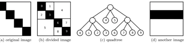
Figure 2(a) presents an example of a binary image of 4 4× pixels. White pixels have a value of 0, whereas black pixels have a value of 1. The rank of the matrix representing this image is r=4 since no row or column is linearly de-pendent on the other. Figure 2(b) presents a partitioning, in which only pixels of the same intensity were kept together. The quadtree corresponding to the di-vision performed is illustrated in Figure 2(c).
[image:5.595.215.537.629.706.2]Since all regions have pixels of the same intensity, the rank of each region in Figure 2(b) is equal to r=1. Figure 2(d) presents an image where 4 pixels are black, but with another configuration. This image has rank r=1, which shows a dependence of the rank and, consequently, of the good performance of the SVD in relation to the image content.
DOI: 10.4236/jsip.2019.103005 64 Journal of Signal and Information Processing The number of units (number of values) required to store the SVD matrices can be expressed as
Units= +r pr nr+ (9)
where r is the rank, whereas p and n are the dimensions of the original image. The first term of the sum (r) corresponds to the diagonal matrix size Σ,
whe-reas the other values correspond to the two other matrices U and V. Thus, the number of units needed to store the image shown in Figure 2(a) is given by
( )( ) ( )( )
4 4 4+ + 4 4 =36 (10)
On the other hand, for the image after partitioning, illustrated in Figure 2(b), the number of units can be calculated as
( )( ) ( )( )
( )( ) ( )( )
( )( ) ( )( )
1 2 1 2 1 5
1 1 1 1 1 3
5 2 3 8 34
+ + =
+ + =
+ =
(11)
We note that, for this division in the image, the number of units needed to store the SVD matrices has decreased. The amount of units needed to store SVD matrices with the division (considering all divisions with the same rank) is smaller than in the entire image, since
(
)
(
)
4
2 2
4 2 2
2 1 2 1
2 2
1
p n
r r r r pr nr
r pr nr r pr nr
r p n r r p n
r r
p n
′+ ′+ ′< + +
′+ ′+ ′< + +
′ + + + ′< + +
′ + <
+ +
(12)
where r′ is the rank of the matrices after division and r′ is the rank of the
original matrix.
In our method, we determine the best alternative, that is, whether the decom-position will be calculated in the entire image or in its four blocks, from the op-timal value calculated with Equation (2). Thus, the block division will be chosen if
4
0opt_value opt_value
4 j j=
>
∑
(13)where opt_value is the optimal value for the entire image and opt_valuej is the optimal value for the j-th block.
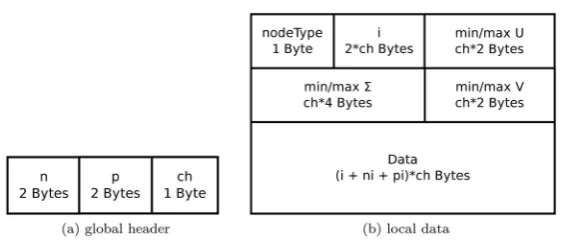
For color images, a decomposition is calculated separately for each color channel. Finally, having the necessary information, the compressed image is stored in a binary file. Figure 3 shows the protocol used to store the image, with header and data.
DOI: 10.4236/jsip.2019.103005 65 Journal of Signal and Information Processing
Figure 3. Image representation in a binary file.
and the number of channels (ch) of the image. They determine the size of each node in the tree, which is necessary to correctly retrieve the data in the decom-pression step.
The tree nodes are stored, as shown in Figure 3, having a local header and data. The first information in this header is the type of node: 1) internal or 2) leaf. For internal nodes, we do not have data, but four children. Thus, after an internal node, four other nodes are expected. For the leaf nodes, besides the node type, we have the rank value r, the minimum and maximum values of each of the matrices. Finally, we have the data for that particular node.
Given the compressed image, the file is read and the tree is reconstructed. For each SVD matrix, a linear transformation is applied in order to return it to the original interval. This is done by using Equation (8), where, in this case, fmin
and fmax are 0 and 255 and gmin and gmax are the various minimums and
maximums of the original matrix. Next, we apply a transformation inverse to that made in Equation (7) to retrieve the decimal values. Finally, the matrices are multiplied to obtain an uncompressed image.
3.2. Evaluation Metrics
We evaluated the compression under two different aspects: the size of the com-pressed image and the quality of the uncomcom-pressed image. For the first, we adopted the compression rate that can be expressed as
( )
( )
S I S
S I
=
′ (14)
where S I
( )
refers to the size of the uncompressed image in bytes, whereas( )
S I′ refers to the size of the compressed image in bytes. The result of this
measurement indicates how many times the compressed image is smaller than the original image.
To evaluate the quality of the decompressed image, we used the mean of the structural similarity index (MSSIM), expressed as
( )
0SSIM ,(
)
MSSIM ,k
i i
i I J
I J
k
=
=
∑
(15)DOI: 10.4236/jsip.2019.103005 66 Journal of Signal and Information Processing
i
J are the i-th windows of the images and k is the total number of windows. The structural similarity index (SSIM) [36] is expressed as
( )
(
(
)
)
(
(
)
)
(
)
(
)
(
(
)
)
2 2
1 max 2 max
2 2
2 2 2 2
1 max 2 max
2 2
SSIM , x y xy
x y x y
k L k L
x y
k L k L
µ µ
σ
µ
µ
σ
σ
+ + + +
=
+ + + + + + (16)
where µx and µy are the means of x and y, σx2 and
σ
2y are the variances ofx and y. The variable
σ
xy is the covariance between x and y, whereas k1 and 2k are constants. The SSIM values are in a range of
[
−1,1]
, where the higher the value, the greater the similarity.4. Experimental Results
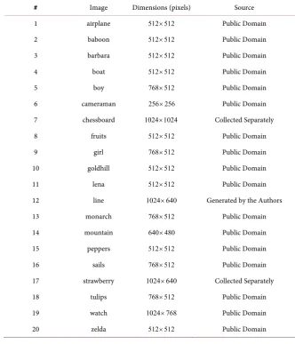
[image:8.595.205.538.340.728.2]This section presents the results of experiments conducted on a set of twenty input images. Table 1 summarizes some relevant characteristics of the images. Seventeen images were extracted from a public domain repository [37], whereas the other three were collected separately.
Table 1. Images used in our experiments.
# Image Dimensions (pixels) Source 1 airplane 512 512× Public Domain 2 baboon 512 512× Public Domain 3 barbara 512 512× Public Domain
4 boat 512 512× Public Domain
5 boy 768 512× Public Domain
6 cameraman 256 256× Public Domain 7 chessboard 1024 1024× Collected Separately 8 fruits 512 512× Public Domain
9 girl 768 512× Public Domain
10 goldhill 512 512× Public Domain
11 lena 512 512× Public Domain
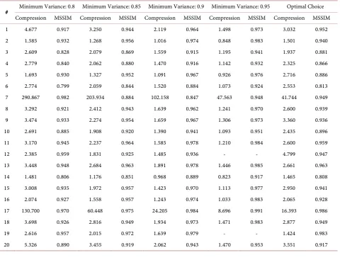
DOI: 10.4236/jsip.2019.103005 67 Journal of Signal and Information Processing In the experiments performed, we compared the relationship between the compression ratio and the MSSIM value. Initially, Table 2 presents different strategies for choosing the σi eigenvalue. The first strategy, used in other ap-proaches available in the literature [34], considers a minimum variance to be preserved in the image. Thus, the eigenvalue σi is chosen so that the variance maintained by the eigenvalues σ1, ,σi is greater than or equal to the mini-mum variance, whereas the second strategy chooses an optimal eigenvalue σi, as defined in Equation (2).
[image:9.595.61.542.367.734.2]We can notice that the results obtained by the optimal choice have a compres-sion ratio always greater than 1, in order to obtain a smaller image in all cases, and with high MSSIM values. Since different images have different variance, re-quiring different amounts of eigenvalues to obtain the same variance, as dis-cussed in Section 0, the minimum variance cannot be used as a fixed value. For example, for images #1 and #5, the compression ratio is less than 1 with variance 0.95, whereas, for image #14, maintaining a variance of 0.9 has already caused the compression ratio to be less than 1. This demonstrates the need to make an adaptive choice. Figure 4 compares the different versions obtained for image #17.
Table 2. Comparison between minimum variance and optimal choice.
DOI: 10.4236/jsip.2019.103005 68 Journal of Signal and Information Processing
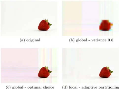
Figure 4. Result comparison for image #17.
It can be observed that, despite a considerably high result in the MSSIM of the global version with variance 0.8 (0.970), the visual result, shown in Figure 4(b), is very poor, whereas the results are superior with the optimal choice, however, still having some problems.
The artifacts that can be seen in Figure 4(c) occur mainly due to the rounding and linear transformation defined in Equations (7) and (8). This problem can be overcome by a more local strategy, such as the one adopted in this work and with the result shown in Figure 4(d). This improvement probably occurs since the values obtained from the matrices after the decomposition are in a smaller range and closer to 0 to 255, because they have a smaller variation in the image.
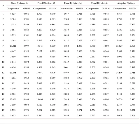
As discussed in Section 0 and observed from the previous results, the SVD technique applied globally may not be adequate. Thus, Table 3 presents the re-sults obtained by considering the image divided into square blocks of different sizes. In addition, it presents the results obtained with the method presented in this work, that is, with the adaptive choice of blocks and eigenvalues.
Comparing the results obtained with those shown in Table 2, overall, the compression rates of the images increased, maintaining high MSSIM values. This demonstrates the validity of the local division strategy which, in addition to the reduction of the artifacts shown in Figure 4(c), obtains better quantitative results.
The compression and MSSIM values obtained with the adaptive division are generally similar to those obtained with the fixed block size. However, for image #7, which consists of a chessboard, the result obtained is considerably superior in terms of compression ratio, which demonstrates superiority of the adaptive division. This result can vary considerably in different images with the change of the constant values given in Equation (6). The values used were chosen empiri-cally in order to obtain a good result in all images.
DOI: 10.4236/jsip.2019.103005 69 Journal of Signal and Information Processing of the image are lost in the compression process. In this case, this occurs most notably with a smaller block size. This is an apparent limitation of our adaptive division, which could select a larger block size in those regions, in order to pre-serve more detail. In order to circumvent this problem, we could choose a more suitable value for α, used in Equation (2), or limit the minimum size of the block adaptively.
Figure 5. Result comparison for image #4.
Table 3. Comparison between fixed and adaptive block partitioning.
DOI: 10.4236/jsip.2019.103005 70 Journal of Signal and Information Processing It is noteworthy that the requirements for storing the compressed images could still be reduced. For example, a flag used to determine the node type could be only 1 bit long, instead of 1 byte as employed in our implementation for sim-plification purposes.
5. Conclusions
This work described and implemented a new lossy image compression method based on the singular value decomposition. The proposed approach used an op-timal choice of eigenvalues computed in the decomposition, as well as an adap-tive block partitioning. We also presented a protocol for storing the SVD ma-trices.
Experiments were conducted on a dataset composed of twenty images—se- venteen extracted from a public domain repository and commonly used in the evaluation of image processing tasks, the other three images collected separately. The results obtained show that the optimal choice of eigenvalues is relevant due to differences in different image contents.
Due to rounding performed in the compression process, the overall approach achieved lower compression rate and added artifacts to the images. In addition, the adaptive partitioning strategy obtained, in some cases, considerably superior results in terms of compression ratio. However, some fine image details may be lost in the compression process based on local strategy.
Acknowledgements
The authors are thankful to São Paulo Research Foundation (FAPESP grants #2017/12646-3 and #2014/12236-1) and National Council for Scientific and Technological Development (CNPq grant #309330/2018-1) for their financial support.
Conflicts of Interest
The authors declare no conflicts of interest regarding the publication of this pa-per.
References
[1] Cho, Z.-H., Jones, J.P. and Singh, M. (1993) Foundations of Medical Imaging. Wi-ley, New York.
[2] Jensen, J.R. and Lulla, K. (1987) Introductory Digital Image Processing: A Remote Sensing Perspective. GeocartoInternational, 2,65.
https://doi.org/10.1080/10106048709354084
[3] Crocker, J.C. and Grier, D.G. (1996) Methods of Digital Video Microscopy for Col-loidal Studies. JournalofColloidandInterfaceScience, 179, 298-310.
https://doi.org/10.1006/jcis.1996.0217
DOI: 10.4236/jsip.2019.103005 71 Journal of Signal and Information Processing 91-109. https://doi.org/10.1007/0-306-47815-3_5
[5] Andrews, H. and Patterson, C. (1976) Singular Value Decompositions and Digital Image Processing. IEEETransactionsonAcoustics, Speech, andSignalProcessing, 24, 26-53. https://doi.org/10.1109/TASSP.1976.1162766
[6] Bhavani, S. and Thanushkodi, K.G. (2013) Comparison of Fractal Coding Methods for Medical Image Compression. IETImageProcessing, 7, 686-693.
https://doi.org/10.1049/iet-ipr.2012.0041
[7] Messaoudi, A. and Srairi, K. (2016) Colour Image Compression Algorithm Based on the DCT Transform Using Difference Lookup Table. Electronics Letters, 52, 1685-1686. https://doi.org/10.1049/el.2016.2115
[8] Qureshi, M.A. and Deriche, M. (2016) A New Wavelet Based Efficient Image Com-pression Algorithm Using Compressive Sensing. Multimedia Toolsand Applica-tions, 75, 6737-6754. https://doi.org/10.1007/s11042-015-2590-9
[9] Yao, J. and Liu, G. (2017) A Novel Color Image Compression Algorithm Using the Human Visual Contrast Sensitivity Characteristics. PhotonicSensors, 7, 72-81. https://doi.org/10.1007/s13320-016-0355-3
[10] Prakash, A., Moran, N., Garber, S., Dilillo, A. and Storer, J. (2017) Semantic Per-ceptual Image Compression Using Deep Convolution Networks. 2017 Data Com-pressionConference, Snowbird, UT, 4-7 April 2017, 250-259.
https://doi.org/10.1109/DCC.2017.56
[11] David, M., George, T., Michele, C., Troy, C., Nick, J., Joel, S., Hwang, S.J., Vincent, D. and Singh, S. (2017) Spatially Adaptive Image Compression Using a Tiled Deep Network. 2017 IEEEInternationalConferenceonImageProcessing, Beijing, 17-20 September 2017, 2796-2800. https://doi.org/10.1109/ICIP.2017.8296792
[12] Zhang, Y., Xu, B. and Zhou, N. (2017) A Novel Image Compression-Encryption Hybrid Algorithm Based on the Analysis Sparse Representation. Optics Communi-cations, 392, 223-233. https://doi.org/10.1016/j.optcom.2017.01.061
[13] Zhao, C., Zhang, J., Ma, S., Fan, X., Zhang, Y. and Gao, W. (2017) Reducing Image Compression Artifacts by Structural Sparse Representation and Quantization Con-straint Prior. IEEETransactionsonCircuitsandSystemsforVideoTechnology, 27, 2057-2071. https://doi.org/10.1109/TCSVT.2016.2580399
[14] Ahanonu, E., Marcellin, M. and Bilgin, A. (2018) Lossless Image Compression Us-ing Reversible Integer Wavelet Transforms and Convolutional Neural Networks. 2018 DataCompressionConference, Snowbird, UT, 27-30 March 2018, 395-395. https://doi.org/10.1109/DCC.2018.00048
[15] Toderici, G., Vincent, D., Johnston, N., Hwang, S.J., Minnen, D., Shor, J. and Co-vell, M. (2017) Full Resolution Image Compression with Recurrent Neural Net-works. ConferenceonComputer Visionand PatternRecognition, Honolulu, HI, 21-26 July 2017, 5435-5443. https://doi.org/10.1109/CVPR.2017.577
[16] Baxes, G.A. (1994) Digital Image Processing: Principles and Applications. Wiley, New York.
[17] Sayood, K. (2017) Introduction to Data Compression. Morgan Kaufmann, Burling-ton, MA.
[18] Nelson, M. and Gailly, J.-L. (1996) The Data Compression Book. M & T Books, New York.
[19] Gonzalez, R.C. and Woods, R.E. (2002) Digital Image Processing.
DOI: 10.4236/jsip.2019.103005 72 Journal of Signal and Information Processing [21] Sharma, M. (2010) Compression Using Huffman Coding. InternationalJournalof
ComputerScienceandNetworkSecurity, 10, 133-141.
[22] Connell, J.B. (1973) A Huffman-Shannon-Fano Code. ProceedingsoftheIEEE, 61, 1046-1047. https://doi.org/10.1109/PROC.1973.9200
[23] Gonzales, C.A., Anderson, K.L. and Pennebaker, W.B. (1990) DCT-Based Video Compression Using Arithmetic Coding. Electronic Imaging: Advanced Devices and Systems,Santa Clara, CA, 1990, 305-312. https://doi.org/10.1117/12.19522
[24] Morita, H. and Kobayashi, K. (1989) An Extension of LZW Coding Algorithm to Source Coding Subject to a Fidelity Criterion. 4thJointSwedish-SovietInt. Work-shoponInformationTheory, Gotland, Sweden, 105-109.
[25] Pountain, D. (1987) Run-Length Encoding. Byte, 12, 317-319.
[26] Rabbani, M. and Jones, P.W. (1991) Bit Plane Encoding. In: DigitalImage Com-pressionTechniques, SPIE Press, Bellingham, WA, 49-62.
[27] Jain, A.K. (1981) Image Data Compression: A Review. ProceedingsoftheIEEE, 69, 349-389. https://doi.org/10.1109/PROC.1981.11971
[28] De Jager, F. (1952) Delta Modulation, a Method of PCM Transmission Using the 1-Unit Code. PhilipsResearchReports, 7, 23.
[29] Schindler, H. (1974) Linear, Nonlinear, and Adaptive Delta Modulation. IEEE TransactionsonCommunications, 22, 1807-1823.
https://doi.org/10.1109/TCOM.1974.1092119
[30] Rao, K.R. and Yip, P. (2014) Discrete Cosine Transform: Algorithms, Advantages, Applications. Academic Press, Cambridge, MA.
[31] Lewis, A.S. and Knowles, G. (1992) Image Compression Using the 2-D Wavelet Transform. IEEETransactionsonImageProcessing, 1, 244-250.
https://doi.org/10.1109/83.136601
[32] Watson, A.B. (1994) Image Compression Using the Discrete Cosine Transform.
MathematicaJournal, 4, 81.
[33] Waldemar, P. and Ramstad, T. (1997) Hybrid KLT-SVD Image Compression. 1997
IEEE International Conference on Acoustics, Speech, and Signal Processing, Mu-nich, 21-24 April 1997, 2713-2716.
[34] Rufai, A.M., Anbarjafari, G. and Demirel, H. (2014) Lossy Image Compression Us-ing SUs-ingular Value Decomposition and Wavelet Difference Reduction. Digital Sig-nalProcessing, 24, 117-123. https://doi.org/10.1016/j.dsp.2013.09.008
[35] Wang, Z., Bovik, A.C., Sheikh, H.R. and Simoncelli, E.P. (2004) Image Quality As-sessment: From Error Visibility to Structural Similarity. IEEETransactionson Im-ageProcessing, 13, 600-612. https://doi.org/10.1109/TIP.2003.819861
[36] Hu, Y.H. (2018) Public-Domain Test Images.
https://homepages.cae.wisc.edu/~ece533/images/index.html
[37] Ranade, A., Mahabalarao, S.S. and Kale, S. (2007) A Variation on SVD Based Image Compression. ImageandVisionComputing, 25, 771-777.