A thesis presented for the
degree of Doctor of Philosophy in Physics in the University of Canterbury,
Christchurch, New Zealand.
by
G.J. FRASER
T�ESIS 'VQc
�19
. F io4\v t> \ • I �op�\
The greater wave is covered wi�h innumerable other waves which move in different directions; and these are deep or shallow according to the power that generated them ••••••••
In an attempt to make synoptic observations of winds in the mesosphere and lower thermosphere, a simpli fied version of the correlation method for analysing spaced receiver ionosphere drift observations was devel oped. The new method makes possible the use of much simpler recording methods and eliminates the manual reduction of records. Drift observations made at noon between altitudes of 65 and 100 km, for summer 1963-4 and winter 1964 are presented. It is concluded that the mean monthly drift is a good estimate of the winds at these heights. The most prominent feature of the seasonal circulation is the upward progression of the height of reversal from westerlies (below) to easterlies
ACKNOWLEDGEMENTS.
The research described in this thesis is part or the research programme of the University of Canterbury Physics Department, and I wish to thank Professor A.G. McLellan for his interest in the project.
I also wish to thank Dr. J.B. Gregory, for the generous as istance and advice which he provided during the course of the experiment.
The technical assistance so necessary to the success of the experiments was provided primarily by Mr. A.W. Black and Mr. B.A. Perry with help from other members of the Physics Department Staff and occasional student labour.
I must also thank the trustees of the estate of the late Mr. A.E. Birdling for generously providing a field site, which has proved a most spacious and noise free environment for the experimental work.
Since the computer is necessarily so much a
part of the experimental techni�ue I must thank Professor D.F. Lawden of the Mathematics Department and Mr. B.A.M. Moon of the University of Canterbury Mobil Computer
ically reproduced by Mr. E.R. Mangin. Many of the
individual wind profiles were plotted by Mr. J. Macinnes.
CONTENTS
1 • INTRODUCTION.
2. GROUND-BASED RADIO OBSERVATIONS OF AIR MOTION IN THE UPPER ATMOSPHERE.
2 . 1 • 2.2.
Principles of the method.
The nature of the reflecting surface. Height resolution of the radio method.
CORRELATION ANALYSIS OF THE G ROUND DIFFRACTION PATTERN. 1 6 6
7
10 1 2 3.1. The correlation functions of the fading records. 12 3.2. The application of tetrachoric correlation tothe analysis of fading records. 17 3.3. Calculations for a joint Gaussian probability
4.
4.1 •distribution.
THE DETERMINATION OF THE DRIFT VELOCITY. Introduction to the velocity parameters.
4.2.
Determination of the velocity parameters from the4.
3
.
correlograms.
Velocity parameters when the receivers are not in the line of drift.
4.4.
The analysis of a statistically anisotropic diffraction patte�n.OUTLINE OF EXPERIMENTAL METHOD. Apparatus at Birdling's Flat.
22 27 27 30 35 37 39 39 5.1 . 1. The radio transmitting and receiving equipment. 39
5.1 .2. Signal processing unit. 41
Laboratory. 45 6. FEATURES OF THE EXPERIMENTAL CORRELOGRAMS. 48
6 .1 • S�mpling errors. 48
6.2. The influence of phase drift on the
cross-corre-lograms. 54
6.3. Interference between ordinary and extra-ordinary waves.
Conclusion.
ATMOSPHERIC WINDS BETWEEN 65 AND 100 KM. A note on terminology.
The influence of the geomagnetic field on the movement of ionisation.
7.3.
The diffraction of waves by irregularities in7.3.1.
7
.
3
.
2
.
7
.
4
.
7.5
.
7.6.
8.
8 .1 • 8.2. 8.3. 8.4.
a fluid.
A relatively simple example.
Reflection from atmospheric irregularities. The deduction of atmospheric winds from the experimental results.
Influence of solar tides.
Group path delays in height measurement.
THE DYNAMICS OF THE ATMOSPHERE BETWEEN 65 AND 100 KM.
Basic equations of atmospheric motion. Temperatures between 65 and 100 km. The meridional temperature gradient. The circulation between 65 and 100 km.
8.4.1.
The 60 to 70 km winter westerlies.8.4
.2.
The mid-winter height of reversal in the zonal wind.8
.4.3.
The variation in the height of reversal.8.4
.
4
.
Equinoctial variation in the circulation.8
.
4
.5
.
The summer circulation.9. A DISCUSSION OF MOTION IN THE MESOSPHERE. 10. CONCLUSION.
90
Ao RADIO RECEIVERS. A .1 • "Balun" transf'ormer.
B. 2. 3. 4o 5. 6. 7. 8. 9.
Radio f'requency amplif'iero Mixer.
Intermediate f'requency amplifier. Detector.
Video amplif'ier.
Phase ref'erence channel. Local oscillator.
Phase comparison oscillator. DIGITAL LOGIC ELEMENTS.
B .1 • Design criteria f'or digital logic elements. Def'inition of' logic levels and pulses.
Detailed description of' the basic NOR gate. Additional digital logic elements.
Flip-f'lop. 2. 3.
4.
4-1 • 4.2. 4.3.4.4.
4.5. 4.6. 4.7.Pulse gate.
Monostable multivibrator. Schmitt limiter.
48V pulse amplif'ier. Pulse converter.
EXCLUSIVE OR circuit. 4.8. Emitter f'ollower. 4.90 Diode limiter. 4.10. Diode clamp. 4.11 o Power f'lip-f'lop. 4.12. Solenoid driver.
104 104 105 105 105 106 107 107 108 109 11 0 11 3 11 9 129 130 130 131 132 132 132 133 133 133 1 33
c.
D.
E.SIGNAL PROOEBSING
UNI
T
.
PAPER TAPE PUNCH DRIVE UNIT.
HEIGHT GATE GENERATOR.
- introduced on page A output amplitude of receiver intermediate frequ
ency amplifier
Ar amplitude of coherent detector phase reference waveform
13
14 a probability in tetrachoric correlation table 20
a a constant (equation B.4 only) �23
a (x) Gauss function of a normalised variable (x) 24
b probability in tetrachoric correlation table 20
b a constant (equation B.4 only) 123
C reference level for tetrachoric correlation 19 c probability in tetrachoric correlation table 20 D delay bit from monostable multivibrator 131 d probability in tetrachoric correlation table 20 d a apparent depth of reflecting layer 11 d0 spacing between receiver aerials 32 d s thickness of spherical shell (determined by the
width of the transmitted pulse)
E electric field strength of electromagnetic wave E0 amplitude of reflected field strength at receiv
ing aerial
f G g s H HG
(= Fx, FY, Fz) force acting on air mass Coriolis parameter (2h sin
¢
1)receiver gain
gravitational constant atmospheric scale height height gate output bit
Hn (x) Hermite polynomial 24 h (in Section 2.3 only) height of reflecting layer 10 h (in Section 3 only) normalised reference level 23 h (Section 8) earth's angular velocity 81 hFE large signal short circuit forward current
transfer ratio
Ia, I1, I2,
r
3,r
4 input currents to NOR gate I C collector currentI co base-collector junction leakage current IN1, IN2, IN3, IN4 input bit to NOR gate I p base bias current from base supply
i suffix, usually used to distinguish between the three receiving aerials
j suffix, usually used to distinguish between the three receiving aerials
k normalised reference level
L integral of bivariate Gaussian probability distribution
N C
n OUT
critical electron density
electron density at reflection height electron density at ground level
phase refractive index of electromagnetic wave output bit from NOR gate
P, P' reference points (Section 4) p probability (in Section 3 only) p pressure
Yule's coefficient of association Yule's coefficient of colligation
Pearson R a
r r
r m
input resistance in NOR gate base bias resistance in NOR gate correlation coefficient
distance (equation 3.7 only) cross correlation for�= o
maximum value of cross-correlation
r0 cross-correlation when there is no differential phase error
SIG s T t u u V
receiver output bit standard deviation temperature
time
eastward wind component
dummy variable (in equations 6.1 and 6.2 only) a constant
real part of coherent detector output voltage base supply voltage
VBE (OFF) base-emitter voltage required to turn trans istor OFF
collector supply voltage
VCE (SAT) saturation collector-emitter voltage
V
v'
receiver intermediate frequency output voltage coherent detector phase reference waveform northward wind component
drift velocity of diffraction pattern apparent drift velocity
v ch�racteristic velocity of random diffraction pattern 27 -c
v"'C ·' v' ex
X
fading velocity
eastward component of fading velocity eastward drift velocity component northward drift velocity component
v' v' Quantities analagous to apparent drift velocity x' Y
w X X X y y z z'
(VI)
upward wind component
height-selected signal bit
eastward displacement co-ordinate
(in Section 3 only) normalised random variable northward displacement co-ordinate
(in Section 3 only) normalised r�ndom variable vertical displacement co-ordinate
virtual reflection height real reflection height
z1, z2 arbitrary height integration limits
o spatial lag (argument of spatial correlation function)
"size" of diffraction pattern phase of received wave
latitude
phase error in receiver
angle between drift vector(�) and x-axis width of transmitter-receiver polar diagram angle used in definition of velocity parameters air density
�k time lag for which the autocorrelation has fallen to rk
time lag for maximum cross-correlation "fading period"
� 01 "fading period" of reflection from a moving rigid surface
�02 "fading period" of reflection from a randomly moving surface with no steady motion
� s time lag for which the autocorrelation has
w
C
fallen to rm
maximum time lag for a given correlation carrier freQuency of received wave
• complex conjugate
< > mean value
Logic functions: • AND
+ OR
- NOT
31 31 16
28
29
1
1 0 INTRODUCTION
Air movement in the upper atmosphere can be observed from the ground by watching the movement of characteristic features in the air mass. At lower levels clouds are the most common natural tracers in the air. Further up, at altitudes of about 80 km, noctilucent clouds have indicated atmospheric movement in that region. The height limitations of the meteor ological sounding balloon have, until recently, prevented the meteorologist from taking soundings in the strato sphere above 30 km. The development of small solid fuel rockets has provided a much more satisfactory
vehicle for carrying instruments to measure the physical properties of the atmosphere. Standard methods of mea suring atmospheric pressure and temperature fail above 50 to 60 km because the sensitivity of aneroid barometers is inadequate for reliable low pressure measurements, and temperature-sensing devices become inaccurate- the heat energy transferred to the thermometer by radiation is no longer negligible compared with the energy transferred by molecular collisions.
are formed at altitudes of 80 to 100 km. Two very
thorough investigations of upper atmosphere winds,
based on this method, have been made by Greenhaw and Neufeld (1961) at Jodrell Bank near Manchester in
England and Elford (1959) at Adelaide, South Australia.
Artificial tracers are now extensively used to follow the air motion at these very high altitudes. Sodium vapour clouds, produced from burners carried
in a rocket, or the smoke trails of rocket motors can
be tracked optically. Radar equipment can be used to
follow the motion of "chaff" (small pieces of metal
foil), parachutes, balloon-supported corner reflectors,
or falling spheres. The macroscopic objects are of
little use above 60 km because the viscous force ex
erted on them by the moving air is less than the grav
itational force� and the objects do not follow the air
movement. This difficulty does not arise with micro-scopic objects like the smoke particles, the vapour molecules, or the electrons and ions in the meteor trails.
One of the most successful radar targets which have been used at altitudes of about 80 km is the ROBIN
(for rocket balloon instrumentation). A thin plastic
3 carried up by a small solid fuel rocket, ejected, in flated and then followed by ground radar. Horizontal motion of the sphere indicates the horizontal component of the wind vector. Since the vertical component of the wind is negligible, the atmospheric density can be calculated from the vertical velocity of the sphere.
Extensive measurements of atmospheric density and winds have been made by Nordberg and his fellow workers (see, for example, Nordberg 1964). They obser ved the ray paths and velocity of the sound waves pro duced when a sequence of grenades is ejected from a rocket as it passes through the atmosphere. Results from various rocket experiments will be discussed in Section 8.
Electrons are the lightest tracers which can be used to study the motion of the ionised gas containing them. Solar radiation is the most common source of
ionisation, and the consequent free electrons in the upper atmosphere. The ionosphere so produced appears as an inhomogeneous, anisotropic, dissipative medium to electromagnetic waves. The inhomogeneities in the
diffraction pattern formed on the ground. This fact is the basis of the experimental work described in out line in Section 2 and in more detail in Sections 3 to 7.
The intensity at any point in the diffraction pattern is a random function of space and time and var ious statistical parameters for describing its behaviour are defined in Section
3.
Section4
shows how the stat istical parameters are used to determine the driftvelocity of the diffraction pattern, and in Section 7 we investigate relationship.between the diffraction pattern drift velocity and winds in the atmosphere between alti tudes of 65 and 100 km. Section 5 is a brief descrip tion of the equipment (details are given in the appendices) and Section 6 discusses the records obtained from the
equipment.
The ionosphere is only a small part of the whole atmosphere, which is a compressible, inhomogeneous fluid on a rotating sphere - the earth. The fluid is·· perturbed by tidal forces, thermally generated circulation systems and various forms of instability. The time
5
appears to be statistically non-stationary, i.e. even its "average" properties are not constant. Any theories of atmospheric motion, or explanations of experimental observations, are therefore severely limited by the approximations which are necessary to obtain a
quanti-tative answer. In Section 8, the equations of atmos-pheric motion are considered and, with the help of certain approximations, used to interpret the experi mental results.
The emphasis throughout this investigation has been to use the diffraction drift experiment as a tool for the synoptic investigation of atmospheric winds above altitudes of 65 to 70 km. The discussion in Section 8 shows that this aim was achieved. The principal techniques which have made this objective attainable are the
(i) use of simplified data recording methods, whose use became evident after an investigation of the minimum amount of information necessitated by the method of correlation analysis
(ii) the elimination of manual data reduction and (iii) the conceptof on- and off- line computing
2. GROUND-BASED RADIO OBSERVATIONS OF AIR MOTION IN TR..E UPPER ATMOSPHERE.
2. 1. PRINCIPLES OF THE METHOD.
After the establishment of radio communications in the early years of this century it soon appeared that there were short-term (compared with diurnal variations) variations in the amplitude of the electromagnetic waves received at a fixed point, from a fixed transmitter. This amplitude variation was called "fading". Appleton and Ratcliffe (1927) investigated the fading of waves received from a transmitter 150 km from the receiver. By using a loop and a vertical aerial to distinguish the ground wave from the wave reflected from the ionosphere,
7 between corresponding maxima and minima, indicating a
translational motion of the diffraction pattern. Mitra
(1949) used three aerials in a triangular array to invest
igate the two-dimensional motion of the diffraction pattern.
Figure 2.1 indicates the basic principles of this spaced receiver method of investigating a drifting diffraction
pattern. Figure 2.1 (�) is a vertical cross-section of
the experiment. The transmitted waves are returned from
the "rough" reflecting surface and produce the diffraction
pattern on the ground. Figure 2.1 (b) is a horizontal
cross-section, with a hypothetical set of contours of
constant electromagnetic field strength. As the pattern
moves across the ground it intersects the receiving aerials and the variations in field strength can be recorded as a
function of time at each of the three points. An analysis
of the field strength variations yields the time delay
between pairfu of receivers, and enables the velocity of the
pattern to be calculated. The methods used are discussed
in Section 3 and
4.
2.2 THE NATURE OF THE REFLECTING SURFACE.
[image:24.517.64.477.63.511.2]c
E + n (z) E = o 2dz2
where n = refractive index
z = distance along the vertical axis E = electric field
strength-( 2 .1 )
The use of ray theory, or the Liouville
(WKBJ)
approximation, requires that1
dn 0n dz
(2.2)
and
1
d2n 02 n dz
If the relative change in refractive index is not negligible
there is a reflected wave.
invalid by two conditions:
Equations (2.2) are rendered
(i) n = o ("total" reflection)
and (ii) dn dz N n ("partial" reflections)
Most of the results to be described utilised partial re flections from the lower parts of the ionosphere where the electron density is low and the refractive index close to
unity. Consequently the rate of change of refractive
9
wave. Since the fractional change in refractiv� index is not large, this change must occur in a very short distance. Albini and Jahn (1961) and Brekovskikh (1960) show curves for calculations on various (simple) theoret ical models for a discontinuity in refractive index.
They find that if the discontinuity extends over a distance of about a half-wavelength or less, the actual shape of the discontinuity is of secondary importance. The reflection coefficient depends primarily on the difference in refract ive index on either side of the discontinuity. A step discontinuity in refractive index is therefore a reasonable model, and a very useful one because the (Fresnel) reflec tion coefficients are easily calculated.
There is evidence that even when the totally reflected waves are considered, irregularities close t0 the point of reflection are the principal source of fading.
The experimental evidence is provided by Jones (1958) who measured the variation of wind velocity with height, using waves of frequency 2.0 and 2.5 Mc/s, each totally reflected from the E layer at an altitude of about 110 km. The
wind measurements at Jodrell Bank. The theoretical evidence is provided by Pitteway (1960).
It can therefore be assumed that the movement of the diffraction pattern on the ground depends on the movement of the irregularities within a small distance, probably of the order of several hundred metres, of the reflection height. This is well within the limits imposed by the height resolution of the eQuipment.
2.3. HEIGHT RESOLUTION OF THE RADIO METHOD.
1 1 cross correlation between two aerials spaced two wave lengths apart, is about 20° (the semi-angle subtendeu bJ the first Fresnel zone is 2.3°).
Thus h sin ed
=
27 km and h cos ed=
75 kmhence d a
=
h - h cos ed=
5 kmThe height limits of the spherical cap are therefore
The height resolution for a uniformly dense scattering region is thus 9 km.
2•
.
CORRELATION ANALYSIS OF THE GROUND DIFFRACTION PATTERN.Standard techniques are available for the analysis of the fading records from spaced receivers. An excellent review of ionospheric diffraction has been given by
Ratcliffe (1956). The most satisfactory techniques (described in Section
4)
necessitates a considerable amount of computing. The purpose of the present study is to investigate synoptically the windE below 100 km, so that methods of analysis must be rapid and convenient.With some approximations and consequent simplifications,
the ease of recording data and the subsequent analysis by correlation techniques can be made acceptable for use in synoptic wind observations.
is discussed in Section 3. 2.
The simplified method
3o1. THE CORRELATION FUNCTIONS OF THE FADING RECORDS.
The physical variable actually measured in the spaced-receiver experiment is the electromagnetic field strength on the ground. The field induces in each aerial an e.m.f. which is amplified by the succeeding radio
receivers. Let the electric field strength at an aerial be
13 Equation (3.1) is the usual expression for a randomly
perturbed wave. It indicates an "almost simple harmonic"
variation of field strength, with an angular frequency w , C
and amplitude and phase terms which are random functions
of time. If the ratio of receiver output voltage to
electric field strength at the aerial is Gs, the receiver
intermediate frequency amplifier output voltage must be
= r w t
� C +
= A (t). exp j co (t). exp j
co (t)J
CJ.) t
C
(
3
.
2)
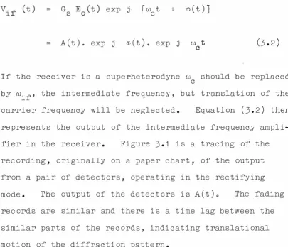
If the receiver is a superheterodyne w should be replaced C
by rJ..lif' the intermediate frequency, but translation of the
carrier frequency will be neglected. Equation (3.2) then represents the output of the intermediate frequency ampli
-fier in the receiver. Figure 3.1 is a tracing of the
recording, originally on a paper chart, of the output
from a pair of detectors, operating in the rectifying
mode. The output of the detectors is A (t)o The fading
records are similar and there is a time lag between the similar parts of the records, indicating translational motion of the diffraction pattern.
[image:30.517.68.473.236.584.2]a reference level for recording (see Section
3.2).
The functionV(t) = Real fA (t) exp j ©(t)l
(3.3)
is the output of a coherent detector with a signal input given by
(
3
.
2
)
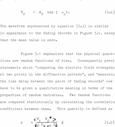
and a phase reference signal ofV r = A exp j r wt. C (3.4)
The waveform represented by equation
(
3
.3)
is similar in appearance to the fading records in Figure 3.1, except that the mean value is zero.Figure 3.1 emphasises that the physical quant-ities are random functions of time. Consequently previou&. statements about "comparing the electric field strengths at two points in the diffraction pattern", and "measuring the time delay between the pairs of fading records" now have to be given a quantitative meaning in terms of the properties of random variables. Two random functions are compared statistically by calculating the correlation coefficient between them.
r
This quantity is defined as
1
[image:31.523.75.474.196.638.2]15 If the two random variables are identical,
r = 1. If they are "mirror images" r = -1 and if they are independent functions, r
=
0 (but if r=
O, they are not necessarily independent functions).If two of the aerials in Figure 2. 1 (b) are in a line parallel to the velocity of the diffraction pattern, and the diffraction pattern does not change as it moves, the fading records of the two receivers connected to these aerials will be identical, but there will be a time dis-placement. Consequently r / 1 • However if one fading record is shifted by an amount corresponding to the time delay, r = 1. Equation (3.5) is therefore generalised
to allow for a time difference:
r .. lJ ( '"L") = < V . ( t ) • V . * ( t + l 't )>
1
� V. 2 ( l t )> • < V . 2 ( t ) > ) 2
J (3 .6)
Equations (3.4) and (3.5) are limiting forms of (3.6). The numerator of (3.6) is called the covariance; if j = i
it is the usual variance of V., sometimes called the auto-l covariance. A graph of r against '"L" is known as a correlo -gram; if i = j it is an autocorrelogram, and if if j it is
a cross-correlogram. The function r .. ll
h)
is known as an autocorrelation function, and r .. ('"L") is a cross-correlation lJ functton, of the lag '"L". (Examples of auto- andshort catalogue of jargon, we can now proceed to discuss Quantitatively the characteristics of the diffraction pattern formed on the ground by electromagnetic waves
reflected from the random irregularities in the ionosphere.
The diffraction pattern is two-dimensional and changes with time. The average characteristics of the time variations are described by the time correlation function
(3.6),
and the average characteristic of the spatial Quantities can be described by the space correl ation function�r .. (o) lJ --< V. l (r) • V . J * (r + o )>
2 2 1
(<V. (r) >< V . (r) >) 2
]. J
(3.7)
EQuation
(3.7)
describes the average properties of the diffraction pattern along a line in the ground plane. Both the time(3.6)
and space(
3
.
7)
correlation functions provide a measure of the time and space scale of thediffraction pattern. Commonly the time lag, � , such 0 that r (� = 0.5 is called the "fading period". Similarly the spatial displacement, 60, such that
17 the observation points. The calculations of all the time and space correlation functions which would be necessary to define the diffraction pattern in detail would occupy an unreasonable amount of time and require an enormous amount of experimental equipment to record the observations. The two space dimensions of the
ground diffraction pattern and the time dimension can be combined to give a three-dimensional correlation function, with contours of constant correlation forming a three dimensional surface.
3.2. THE APPLICATION OF TETRACHORIC CORRELATION TO THE
ANALYSIS OF FADING RECORDS.
In the correlation analysis of the fading records from three spaced receivers the three cross- correlation functions must be computed for a large number of lags.
At least one of the autocorrelation functions must also be computed, but a better estimate is obtained if all three are computed and their average used. A considerable
amount of computing is necessary to produce all these
correlograms and the purpose of this section is to consider how we may retain the advantages of the correlation analysis without the considerable amount of labour and computer time normally required.
method are
(1) Recording of the three field strength variations on photographic film or pen recorder chart.
(2) Manual reading of these films or charts and the recording of the values in a form suitable for calculation or input to a computer.
(3) Computation of the correlation functions, manually or by means of an electronic digital computer.
We can eliminate the alternative in (3) because manual computation is out of the question. It takes several days to produce a set of correlograms from a
10 minute observation. The correlation analysis can only be used if a computer is available. The manual reduction of records (step 2) is as lengthy a process as the manual computation and is subject to error. This step can be eliminated altogether if the experimental apparatus records the information in a form suitable for input to a computer. Punched paper tape was selected as the recording medium because it is more satisfactory for field use than magnetic tape. Paper tape punches and the associated equipment are also cheaper to operate and more readily available than the equivalent magnetic recording apparatus.
19
shall be recorded on paper tape, we must decide on a
method. An obvious approach is to use one or more digital voltmeters, with their accompanying scanning and programming units. However, apart from the high cost of such complex equipment, there is the problem of maintaining it at a field site.
Fortunately, the digital voltmeter (s) and assoc iated equipment are unnecessary as investigations of the cross-correlation functions of distorted functions (Lawson and Uhlenbeck 1950, Bussgang 1952, Heaps 1962), show that, provided the joint probability distribution of the two
waveforms is known, there is no information lost even if the two functions have been badly distorted by the receiving equipment. We shall consider only an extreme form of distortion - complete limiting (hard clipping) of the waveforms. Under these conditions the only information we retain is whether or not the waveforms exceed given
reference levels (denoted by Ci and Cj) which are determined by the equipment. Consequently there is no need for any degree of accuracy in reading the records and the linearity of the receiving equipment is quite unimportant. However another problem is introduced by the necessity to realise
Vi and Vj must be bi-directional signals and can be
obtained from a coherent detector (equation 3. 3). Tetra choric correlation is commonly called polarity-coincidence correlation when C. = C. = O, as the only information l J
required is the sign, or polarity, of the waveform.
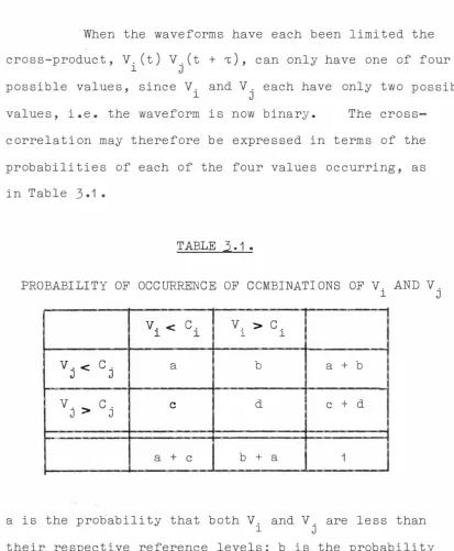
When the waveforms have each been limited the cross-product, V. (t) V . (t + �), can only have one of four l J possible values, since V. and V . each have only two possible l J values, i.e. the waveform is now binary. The
cross-correlation may therefore be expressed in terms of the probabilities of each of the four values occurring, as in Table 3.1.
TABLE 3. 1.
PROBABILITY OF OCCURRENCE OF COMBINATI ONS OF V. AND V.
vi < C . vj < C. J a
V. C. C
J > J
a + C
V. l >
b
d
b + C. l
a
a + b
C + d
1
l J
[image:37.524.58.472.168.669.2]21
that V. l exceeds its reference level while V . J remains below its reference level, and so on. There is only one degree of freedom in this table since the determin
ation of a ,b, c, or d is sufficient to determine the other three quantities (the sums at the sides of the table are determined by the probability distributions of the individ ual waveforms).
We can, of course draw up a table like Table 3. 1 even if we have no information at all about the joint probability distribution of V . and V., or about the res-l J pective probability distributions. Comparisons of this nature are used extensively in analysing qualitative in formation like that obtained in the social sciences or where only two possibities are to be considered, such as the absence or presence of rain (Brooks and Carruthers 1
953
)
.
Early work on this type of comparison has been described by Yule (1900) and Pearson (1901 ). Table 3. 1 is a form of contingency table and various coefficients which can be defined from its entries a, b, c, and d are
(1) Yule ' s coefficient of association
ad - be
(2) Yule ' s coefficient of colligation
Ja:cI -,.Joc
� ad +�be
(3 . 9)
(3) Pearson (1901) defined several more coefficients, among them being
(3.10)
3o3• CALCULATIONS FOR
A
JOINT GAUSSIAN PROBABILITY DISTRIBUTION.If we assume that the joint probability distri bution of the output waveforms (V . (t), V .(t)) of a pair l J of receivers is the bivariate Gaussian distribution
p (V ., V .) = l J exp -2r V . V . V .2� l J + � 2 s . s . s . l J J
(3 . 11 )
2 2
23 levels, C . and C ., i.e. calculate d in Table 3. 1. l J
Simi-larly a, b or c can be calculated. For simplicity, we will assume that the receiver output voltages and reference levels are defined in terms of their respecti ve standard deviations, i.e. write
X = V.
I
s .l l
y = V . J
I
s. J h = C. lI
s . lk = C . J
I
s . J ( 3 . 1 2 )We will also adopt a simpler notation for the integral of the bivariate Gaussian distribution and write
L (h,k,r) �
Jg'.x
f
p(x, y) (3. 13 )Using this notation, the entries in Table 1 are
a = L (-h, -k, r ) b = L (h, -k, r )
L (-h, r) (3.14)
= k,
d = L (h, k,
r)
the experimental results to construct a tetrachoric table, and· then looking up a suitable set of tables of L (h, k, r) such as those in the National Bureau of Standards Applied Mathematics Series (NBS 1959). As the purpose of this thesis is to discuss rapid methods of finding values of correlation, the looking-up of tables is of no further interest. The necessary table look-up could be performed by a digital computer but the storage requirements are excessive. If a digital computer is available, it is possible to calculate L (h, k, r) using a series expansion and to find r by an iterative process. A suitable series, which always converges, is (Kendall and Stuart 1961)
L(h, k, r) = j =oO
j
� �, H. 1 (h). H . 1 (k). a (h). a (k)
j =O J . J - J - (3. 15)
where a (x) = (2�)-1/2 exp (-x2/2) (3.16)
and the H's are the Hermite polynomials:
H (x) = 1
H1 (x) = X H2(x) = X -1
Hn (x) = xHn_1 (x) - (n-1) Hn_2 (x). ( 3 . 1 7 )
is
be measured in the equipment as they can be calculated from the mean values of x and y, once the gains of the receivers have been made equal.In the limit, when h = k = O, (3.13) reduces to
L (O, O, r) = -2 sin r . -1
whence r = sin � [L (O, O,r) ]
and equations (3. 14) become
a = L (-0,
-o,
r) b = L (O, -0, r)C = L (-0,
o ,
r) d = L (O , O, r) Hence a = dand b = c
=
= L (O,
o ,
L (O,
-o,
(3.18)
r)
r)
The coefficients defined by Yule and by Pearson then become
Q1 a2 2 - b2 + b
2
a ( 3 o 1 9 )
Q2 = a - b
a + b (3.20)
Q3 = sin ?C(a - b)
Pearson (1901) studied 15 sample data pairs and found that there was considerable disagreement between
the correlation coefficient calculated in the normal way and the tetrachoric correlation defined by Q1, the mean error over 15 samples being 24 per cent. He did not consider Q2, but found that Q3 had an error of only 4 per cent. Q3 is exact for a joint Gaussian probability dis -tribution, and many physical processes are known to approx
imately obey such a distribution law.
Rice (1944, 1945) deduced the probability dis-tribution of a narrow-band random waveform. The in phase and quadrature components which are A (t) cos co (t) and A (t) sin co (t) respectively, using the notation of equation (3 o 2), each have a Gaussian probability distri-bution. The coherent detection system therefore has an output voltage with a Gaussian probability density function. The detector is then succeeded by the amplifiers and
SECTION
4.
THE DETERMINATION OF THE DRIFT VELOCITY4o1. INTRODUCTION TO THE VELOCITY PARAMETERS.
27
The velocity of the drifting diffraction patte rn can be dete rmined from the correlograms b y the method
discussed below. The discussion is adapted from the paper by Briggs, Phillips and Shinn (1950).
The diffraction pattern m ove s over the ground as the properties of the diffracting screen vary. Its detailed st ructure is als o sub ject to random changes.
The true motion of the drifting diffraction pattern is given by the vector
V = ( v , V )
X y (4 . 1 )
The proportionally constant v was labelled C the characteristic velocity by Briggs, Phillips and Shinn
(1950). They labelled the vector
v ' = (v , v , v )
H C X y C
(
4
.
2
)
the fading velocity (see Figure 4.1 (b).
The signifiance of the fading velocity v ' and C its three components is best shown by considering an observer at the origin of the axes in Figure 4.1 (a)
(observations can of course, only be made in the ground (x, y) pla,ne). If the diffraction pattern has no trans-lational motion and there are no random variations with time (i.e. vc = O), the observer sees a constant amplitude.
29 amplitude variation parallel to the direction of motion are then related by the velocity of the drifting pattern
2 2 .1. V = (v + V )2
X y
= 60 / �01
The higher the drift speed, the faster the fading.
(4.3)
In contrast we can consider reflections from a turbulent reflecting medium with no mean horizontal motion. Then v = v = X y 0. The observer measures a fading period
(�02) characteristic of the random motion and the charact eristic velocity is, by its definition, ( o0 / �02). The diffraction pattern size (q,) will, in general, depend on the direction in the (x, y) plane along which the measure ments are made.
In reality the diffraction pattern changes as it drifts past the observer and the ratio of pattern size
( o0), measured parallel to the direction of drift, to the observed fading period (�0) defines the fading velocity.
v' c = oo
I
�o (4.4)The fading velocity (v' ) C comprises two parts (see equation
(4 . 2 ) )
- a component (v) due to the driftmotion of the diffraction pattern and a component ( V C ) due to random changes in the diffraction pattern. C
on-sequently if an observer moves across the ground plane,
his speed relative to the diffraction pattern is a min imum when he moves with the same velocity as the drift component of the diffraction pattern and all he sees is the random fading represented by v . C Conversely if the observer moves with such a velocity that he sees a max imum fading period, indicating a minimum fading velocity, his velocity must be equal to the drift velocity (v) • This fact provides us with a definition of the drift velocity in terms of observable quantities. This def -inition of the drift velocity (v) also provides the H
definition of the characteristic velocity (v ) because C the minimum fading velocity, as measured by the moving observer, is just V C •
4.2 . DETERMINATION OF THE VELOCITY PARAMETERS FROM THE CORRELOGRAMS.
NOTE In the succeeding sections the distinction
The observable quantities in the correlation analysis are indicated in Figure 4.2(a) which shows
31
the mean auto-correlogram and one cross-correlogram of data recorded on 15 December 1963 at a reflection height of 76 km. It will be assumed, as in the Briggs, Phillips and Shinn (1950 ) paper, that the diffraction pattern in the ground plane is statistically isotropic, i.e. the pattern size. (00) is independent of direction. It will also be assumed that the two receivers are parallel to the drift velocity vector (v ). H � The latter assumption
is invalid for the particular correlograms of Figure 4.2(a) but provides us with a simplified picture so that the
principles of the correlation analysis may be more easily explained. The observable quantities used in the analysis are
the time delay for maximum cross-correlation (r ) m
rk the cross-correlation at zero time delay
�k the time delay at which the autocorrelation has fallen to rk
and � s the time delay at which the autocorrelation has fallen to r
These parameters are shown in Figure 4.2(a).
constant correlation in the ( o , �) plane, as shown in Figure 4.2 (b). It is assumed that the time and space correlation functions have the same shape, although this shape (i.e. the exact form of the correlation functions) need not be known. The ellipses of constant correlation must therefore be concentric and have a constant axial ratio. Figure 4.2(b) can be thought of as a bird's-eye view of a hill whose horizontal cross sections are the correlation ellipses , and whose peak is the origin with a maximum correlation value of 1
.o.
The auto-correlo -gram of Figure 4.2(a) is thus a vertical cross section of the correlation hill in the plane o = O , and the cross correlogram is a vertical cross-section at O = d0 , the spacing between the two receivers whose output signals were compared. The outer ellipse in Figure 4.2(b) is the lower contour r=
rk while the inner one is r=
r • mThe position of the rk ellipse is determined by its inter cepts with the o and � axes at d0 and �k respectively while the inner ellipse must be tangential to the line
0 = d • 0 0 is the intersection of the r ellipse with m m
the 0- axis and is not an observable quantity. From the definition of v'c (equation 4-4) , and the assumption of similar space and time correlation functions, we see that
v '
= d 033
The calculation of the characteristic velocity (v ) follows from the definition given in the previous C section i. e.v
C is the minimum fading velocity that can be observed. The minimum fading velocity corresponds to the maximum fading period for a given correlation value.This value is given by the point of contact between a line of constant time delay tangential to the ellipse for that value of correlation. This time delay is shown as
-i; in Figure 4V .2(b). It is not an observable �uantity.
The correlation appropriate to the spatial separation of d0 in the ground plane must therefore be the same as that produced by a shift of vc-i;v along the -i;-axis. Thus
d 0
-i;v (4 . 6 )
If there was no random component of fading the drift velocity would be that appropriate to the actual receiver separation (d0) and the time lag for maximum
c ros s-c orrelat ion ('t'
m
) • The presence of the random fadingmakes this simple interpretation impossible but we may define another term with the dimensions of velocity.
v '
=
d 0-i; m
(
4
.
7
)
Figure
4.
3
.
It is the velocity of' point P in the ground plane (see equation (4.8) below).The three-dimensional dif'f'raction pattern passes the two receivers placed at O and P in the direction of' the drif't velocity vector (which is here assumed parallel to the x-axis). The characteristic velocity vc has been defined so that the three-dimensional dif'f'raction pattern is statistically isotropic. Maximum cross-correlation thus corresponds to the shortest distance in the dif'f'rac tion pattern , i.e. to the perpendicular distance (PP' in Figure
4.3)
between lines passing through the two receivers in the direction of' v' • .., C The point in the dif'f'raction pattern which was at O when t = 0 has reached P1 in a time -i;m; thenNow
where
OP , = v' c -i;m O'P' = V '];
C ID
QQ 1 = V '];
OP = VI '];
O'P' = PP' cos ev
= OP sin ev cos e
e =
V
-1
tan (O'P'
V
I
oo ' )
(4.8)
(
4
.
9
)
vv' = v2 + v 2
C
35
= (v ' )2
C
(4
.
1
o)v' and v' are defined by e�uations c
(4.
4)
and(4
.
7
)
res pectively so thatV = (v ' )
2
C
v'
X 2 X
=(-o
)I (
_Q )'t"k 't'm
=
X o m 't""b' 2 k
(4. 1 1 )
The velocity defined by e�uation
(4. 1 1 )
is the true translational velocity of the diffraction pattern. The expression is of little use because its derivation was based on the assumption that the two receivers lay on a line parallel to the drift velocity (v). We must next consider how the analysis can be extended to cover the more general situation.4.
3.
VELOCITY PARAMETERS WHEN THE RECEIVERS ARE NOT IN THE LINE OF DRIFT .the line joining the two receivers, its magnitude and direction can only be determined by using a second pair of receivers along a line in a direction not parallel to the first pair. To simpli fy the analysis it will be assumed that the second pair of receivers is at right angles to the first pair, but with suitable tri gonometrical manipulation the analysis can be extended to any combination of receivers. Figure
4
.
4
shows the system of x, y, and v t axis with receivers at O, x and C 0 y0• The analysis to determine the various parameters relative to the x-axis can be carried out as in Section4
.
2
,
except that P is replaced by x0 and the suffix x is used to indicate that measurements are relative to thex-axis. The set of equations corresponding to
(
4
.
8
)
is00 I = V
X X ID
OP ' = v'
1n
C
O' P' = v' (4 .1 2 )
1m
X ex
Ox0 = V I
X
Now cos (P'Ox ) = cos
e
coscpv
0 V
•
oo '
= OP' cos (;z cos <D.
V Vand OP ' = Ox
Thus Oo '
.
Ox = (OP ' )2X 0
00
'
= OO ' cos cpvX
oo '
= Ox coscpv
0
or V V I = (v ' )2·
X X C
V = V C OS cpV X
V I = v ' / cos
cpv
X
similarly Vy V I = (v I )2
y C
V = v sin cp
y V
V I = v ' / sin
cpv
y
The angle ( cpv ) between the
the x-axis is given by
cpv = tan-1 (v ' / v ' ) X
y
dri:ft
and the magnitude o:f the dri:ft vector is
V = (v X 2 + V y 2 ) '�
vector
4.4.
THE ANALYSIS OF A STATISTICALLY ANISOTROPICDIFFRACTION PATTERN.
37
(4 .1 3 )
(4.1 4)
(4. 15 )
(v ) and
(4. 16 )
-tion pattern could be relaxed. They used a procedure similar to that adopted by Briggs, Phillips and Shinn
39
5.
OUTLINE OF EXPERIMENTAL METHOD.The equipment used for the observation of the high altitude atmospheric winds by the diffraction drift method is conveniently divided into two parts
(a ) the radio transmitter, receivers and associated apparatus at the Birdling's Flat field site and (b ) the computer (IBM 1620 ) and associated off-line
equipment in the Mobil Computer Laboratory of the Department of Mathematics, University of
Canterbury.
Only an outline of the apparatus is given here. Details of the electronic circuits are given in Appendices.
5- 1 . APPARATUS AT BIRDLING ' S FLAT.
5.1 .1 THE RADIO TRANSMITTING AND RECEIVING EQUIPMENT.
This is situated at the Birdling's Flat field site (43° 501 S, 172° 40 ' E, 30 km south of Christchurch),
and comprises the following :
(a ) A radio-frequency pulse transmitter generating a 25 micro-second pulse with a peak power of
-1
(b) Transmitting aerial array of 8 half wave ele ments in a broadside array, with a calculated gain of 13.8 dB (relative to an isotropic radiator).
(c) Three receiving arrays, each of two in-phase half-wave elements with a calculated gain of 7.8 dB. They are connected to the receiver by way of 600 ohm open-wire transmission line. The arrays are in the form of a right-angle triangle with sides of 250m (two wavelengths). A spacing of two wavelengths was used. The scale of ionospheric diffraction pattern is so variable that any one spacing will cause re jection of some records in which the cross correlation is too high or too low for satis factory analysis. A spacing of two wavelengths ensures that the rejected observ�tions would be of the smaller scale diffraction patterns,
which could arise from a large random fading component and thus be a poor indication of atmospheric wind motion. It was felt that,
diffrac-41 tion drift method (Barber 1957) but the receiv ing arrays were sited with the possibility of future interferometer experiments in mind.
(d) The three receivers are each preceded by a balun matching unit. For reliability, and with relat ed experiments in mind, it was decided to use three independent receiver channels rather than one channel with diode switches at the input and output. The crystal-controlled local oscill ator is common to all three channels to main tain a constant phase reference at the three coherent detectors. The phase reference sig-nal for the coherent detector is derived from the transmitter crystal oscillator which runs continuously. The receivers also include a video amplifier designed to reproduce the bi directional signals with negligible shift in the d.c. level.
(e) A phase calibration oscillator is necessary to eliminate any systematic phase differences between the three receiver channels. The os cillator and its loop aerial were placed e4ually distant from the three receiving aerials.
5. 1 .2. SIGNAL PR0OESSING UNIT.
between the receiver video stages and the recording de-vice.
The video output signal is first limited about ground potential by cascaded diode and Schmitt limiter
stages.
A
height gate pulse then selects the required part of the reflected waves. The gated signal is at this point a 10 microsecond bit with a repetition period of 20 milliseconds and an amplitude of 12V. Its average power is too low to drive a pen recorder, and it is too short to operate the low speed punch driving circuits.Each signal bit therefore sets a flip-flop which is used as a single-bit storage cell. The flip-flop is reset by each transmitter trigger pulse. In this way the duty
cycle is increased from 0.05 per cent to about 97 per cent.
The fading period of the signals is about 1 to 5 seconds so that there is no need to sample the receiver
-1
outputs more frequently than about 2 sec • In practice -1
a sampling rate of 3.125 sec was used (derived from a
-1
)
50 sec fork and a 4-stage binary divider . With a transmitter pulse repetition rate of 50 sec-1 there is therefore a considerable amount of redundancy in the re-ceiver output signal. It is therefore possible to improve the
The
signal-to-noise ratio by using an integrator circuit. is
43
of 0.05 or 0.25 seconds. The integration increases the rise-time of the binary signal to 2.2 times the integra -tion time constant. To reduce uncertainties in switch -ing levels, this slow signal is again limited about its nominal mean level. A description of the signal process -ing unit , includ-ing a logic diagram appears in Appendix C. Appendix B gives details of the logic elements used.
RECORDERS.
The output from each channel of the signal pro cessing unit has only two values, depending on the value of the limiting amplifier input voltage relative to the reference level. Each observation from each receiver may then be recorded as a single binary digit which has the value 101
, say, when the limiter input is below the
reference level , and the value 11 ' when it is above.
choric tables can be calculated. The recording pro-cess has been simplified although the calculations are complicated by the addition of a decoding operation, but this is of no consequence if a computer is available to carry out the decoding. The decoding required only a small fraction of the total time needed to com
pute the points for the correlograms.
While the paper tape punch control circuits were being constructed a two channel pen recorder was used to record the binary output data from the three receivers. The pen coils were driven by the bridge -connected transistor d.c. amplifiers. By the addition of shunt feedback these were used as summing operationsl amplifiers. As three bits had to be recorded on two channels, the 11' and 121 bits were combined through
the resistive weighting networks of one amplifier to give a O to 3 indication on one channel. The ' 4 ' bit was recorded on the other channel. Even this simple type of chart recording required about 3 man-hours to read for a 10 minute recording time.
45 equipment in the Mobil Computer Laboratory made it des irable to use the standard IBM code, which also has the advantage of representing numbers by their binary-coded-decimal equivalents. The three outputs from the signal processing unit were therefore punched in the 1, 2, and 4 tracks on the tape punch. The punching is carried out by applying the three signals to three pulses gates
-1
which are driven by the 3.125 sec sampling pulse.
The outputs from the pulse gates set (or don ' t set) flip flops in the punch buffer register which drive the punch. Once the character has been punched, a pulse from the punch resets the punch buffer register to await the next pulse. The logical diagram of the paper tape punch drive unit is given in Appendix D.
5.2. EQUIPMENT AVAILABLE IN THE MOBIL_ COMPUTER LABORATORY.
The computer is an IBM 1620 Model 1 with 40,000 digit storage and card input/output. An IBM 870 unit is also available for tape-to-card conversion and graph plotting, in addition to its other functions.
to three time series of binary digits. The tetrachoric correlation function for each point of the correlograms is then calculated, usually from lags of -40 to +40 for the cross-correlation functions and O to + 40 for the autocorrelation functions, with increments of 2 units. The maximum lag and incremental lag can be varied by a program control card. The correlogram points are then punched on to cards in the format required by the IBM Library Autoplotter program which prepares a deck of cards for plotting the correlograms on the modified type writer of the 870.
The correlation program is written in fixed point SPS (a symbolic form of machine language) to ob tain the maximum computing speed. Six correlograms with the lags specified in the previous paragraph, using 150 data digits, are computed in 110 seconds. The same calculation with a Fortran program takes 70 minutes, al though no attempt was made to realise the shortest com puting time with the Fortran program as it was obviously too slow. Normally 500 to 600 data points are used, with a computing time of 4 to 5 minutes.
47
of multiply instructions. As the 1 620 is a serial
binary-coded decimal machine logical operations on
binary data are clumsy and inefficient. The program can be changed to produce the correlograms for 5 1 2 two-digit data points in
6½
minutes, so that the logical instruc tions do shorten the computing time by about 25 per cent. The plotting of the correlogram set takes 1 7 minutes and is the weakest link (in terms of speed) in the chain of calculation.efficient.
A high-speed line printer would be more
6 0 FEATURES OF THE EXPERIMENTAL CORRELOGRAMS.
A
set of experimental correlograms is shown in Figure 6.1. The auto-correlogram and one cross correlogram of this set were used as examples in Section4
.
2
.
The mean auto-correlation function is used because it is found that the three individual auto-correlation functions from the three receivers are not identical. No selection of suitable fading conditions is made at the field site, so that many records consist merely of the noise between pulses reflected from the various altitudes in the atmosphere, and the percentage of useable records is fairly low (40 per oerrt),� The results described in this thesis were obtained from 300 sets of correlograms derived from 740 fading records. It is possible to assess the minimum useable cross-correlation at zero time delay. In future the cross-correlation at zero time delay can be first calculated and if the valuefalls below the minimum the remainder of the correlogram points need not be computed.
6.1. SAMPLING ERRORS.
for the spaced receiver experiment. We must therefore consider the amount of detailed information which it is necessary to retain in the calculations. We have al rea:ly seen (in Section 3.2) that the recording can be simplified because the use of tetrachoric correlation provides ade�uate information for the correlation ana lysis (the actual shape of the space and time autocorr elation functions is of no importance). It will now be shown that there is no need to consider a statisti cally anisotropic ground diffraction pattern and the refinements of the Phillips and Spencer (1955) analysis are unnecessary.
49
The three receivers are each sampling a random function - the amplitude of the electric field in the
diffraction pattern - and sampling errors will be present. The differences between the three time autocorrelation
functions have already been mentioned. The sampling errors also appear as small differences between the cross
correlation values calculated from samples of finite
length. These differences are interpreted by the Phillips and Spencer analysis as anisotropy of the diffraction
pattern, which will introduce errors in the drift velocity if the anisotropy is ignored. It is, however, unreas