of structured random matrices
K. Truong, A. Ossipov
School of Mathematical Sciences, University of Nottingham, Nottingham NG7 2RD, United Kingdom
Abstract.
1. Introduction
Statistical properties of eigenvalues and eigenvectors of random matrices is the central topic of Random Matrix Theory (RMT) [1] . The key idea of RMT is that many features of complex systems are universal and therefore they can be modelled by ensembles of random matrices, which share the same global symmetries, but don’t contain any system specific information. A prominent example of such classical ensemble is the Gaussian Unitary Ensemble (GUE), in which the only constraint is the Hermiticity of a matrix.
Despite the great success of classical RMT during the last fifty years, there is a growing interest to new ensembles of random matrices, in which some structural information about an original system is partly present. In this paper, we study one of such random matrix models, which is defined as
H =WHW˜ +D, (1)
where ˜H is anN×N matrix from GUE andW,D are diagonal matrices with elements
wianddi,i= 1, ..., N, respectively; the matricesW andDcan be either deterministic or
random. Since the presence of the matricesW andDbreaks the unitary invariance of the probability distribution of ˜H, it is reasonable to expect that the statistical properties of the eigenvectors of this model might be very different from the corresponding properties of GUE. How exactly they will be different, is the main question addressed in this work. The random matrices of the form H = LJ R + M, where L, R and M are not necessary diagonal and the random matrix J might be from another random matrix ensemble, appear naturally in various applications including signal processing [2], vibration analysis [3], wireless communication [4] and neural networks [5]. For example, they arise in the linearized dynamics of non-linear neural networks: J is a random connectivity matrix and L,R and M can be expressed through the firing rates and the time constants of the neurons [5]. In the present work we restrict ourselves to the technically simplest case, where L=R and M are diagonal matrices and J is from GUE.
The spectral properties of such random matrices have been studied recently and a number of very general results have been derived (see [5, 6] and references therein), however much less is known about their eigenvectors [7]. In this work, we generalize our recent results, which have been obtained for two particular cases: i) D = 0 and W is deterministic [8] ii) W =I and D is either deterministic or random [9].
One of the main results of this paper is a general non-perturbative, asymptotic expression for the moments of the eigenvectors of H, which allows us to calculate the moments for any given values ofwianddi. From this expression, it follows, in particular,
that the eigenvectorsH remain qualitatively the same as the eigenvectors of ˜H for very generic choice of parameters wi and di. That means, that extended nature of the GUE
small fraction of the available space.
Another important conclusion following from the general result for the moments is that the extended nature of the eigenvectors can be altered, provided that di and wi
become N-dependent. One of the special cases we study in the present paper is the model with D = 0 and uncorrelated Gaussian distributed wi with the variance, which
is N-dependent. Such a model can be considered as a multiplicative counterpart of the Rosenzweig-Porter model [10], whose eigenvectors statistics was calculated in [9]. We find that eigenvectors of this model can be fractal and compute their fractal dimensions. The paper is organized as follows. In Section 2 we derive our general results for the moments of the eigenvectors and the density of states. In Section 3 we investigate a special case of the model with D = 0 and random W. Finally, some conclusions and open problems are discussed briefly in Section 4.
2. Moments of the eigenvectors and the density of states
In this section we derive expressions for the moments of the eigenvectors of H and the density of states. Generally, the local moments at energyE are given by the definition
Iq(n) =
1
ρ(E)
X
α
|ψnα|2qδ(E−Eα)
, (2)
where ψα is a normalized eigenvector corresponding to the eigenvalue Eα and ρ(E) is
the density of states
ρ(E) = 1
N
X
α
hδ(E−Eα)i. (3)
The integer moments can be related to the diagonal matrix elements of the Green’s functions
Iq(n) =
i2−q
2πρ(E)N lim→0(2)
q−1
(GRnn)(GAnn)q−1, q= 2,3, . . . , (4)
whereGRdenotes the retarded Green’s functions and similarlyGAthe advanced Green’s
function, which are defined by
GR/A(E) = (E±i−H)−1, (5)
the derivation can be found in [8]. The superintegral representing the product of the Green’s functions from Eq.(4) is given by
D
GRnn GAnnq−1
E
=
Z
dQ(gaaBB)q−2gBBaa gBBrr + (q−1)garBBgraBB
×exp
(
−N 2StrQ
2−
N
X
i
Str ln(E−iΛˆ−di −wi2Q)
)
.
(6)
Λ = diag(1,1,−1,−1) andgBB = (E−dn−w2nQn−iΛ)−BB1, where the explicit expression
forgBB is given in Appendix A. We notice that the standard action of the superintegral
appearing in the GUE case is altered by the parameters di and wi as expected.
In the limit N → ∞, the integral is dominated by the saddle-points that satisfy the saddle-point equation
Q= 1
N
N
X
i=1
w2
i
E−di−wi2Q
, (7)
where the solutions can be parametrized as [13]
Qs.p. =t+ isT−1ΛT, (8)
the variables s6= 0 and t are two real parameters satisfying the simultaneous equations
t= 1
N
N
X
i=1
w4i(E−di−w2it)
(E−di−wi2t)2+wi4s2
, 1 = 1
N
N
X
i=1
w4i
(E−di−w2it)2+w4is2
. (9)
In this way any physical quantity, which can be expressed through the Green’s functions, can be calculated in terms ofsandtby computing the corresponding superintegral over
T. Then for any given set of parameters{di}and{wi}the above system of the equations
can be solved numerically yielding an explicit result for any quantity of interest. In particular, one can compute the density of states, which takes the form
ρ(E) = s
πN
N
X
i=1
w2
i
(E−di−w2it)2+w4is2
, (10)
and in a similar way, we find the expression for the local moments
Iq(n) =
1 (πρ(E)N)q
sw2
n
(E−dn−w2nt)2+w4ns2
q
Γ(q+ 1), (11)
where Γ(z) is the gamma function andq is a positive integer. These two general results allow us to calculate the density of states and the statistics of the eigenvectors for any particular choice of the matrices W and D in Eq.(1).
Verifying that we recover the GUE case once we set di = 0 and wi = 1 is a simple
exercise, where we obtain
ρGU E(E) = 1
π
p
1−(E/2)2, IGU E
q (n) =
Γ(q+ 1)
6.5 7 7.5 8 −7
−6.5 −6 −5.5 −5
[image:5.612.81.482.99.304.2]ln(
N
)
ln(
I
2)
Figure 1. The symbols represent the numerical simulation and the solid line is our analytical result. The numerical simulation is over 1000 realizations forq = 2 with wi=di=N/i.
these are the well-known results for the GUE case.
Setting wi = 1 we reproduce our previous result derived in [9]:
ρ(E) = s
πN
N
X
i=1
1
(E−di−t)2+s2
,
Iq(n) =
1 (πρ(E)N)q
s
(E−dn−t)2+s2
q
Γ(q+ 1).
(13)
At the same time, we can also recover the result from [8] by setting di = 0:
ρ(E) = s
πN
N
X
i=1
w2i
(E−w2
it)2+wi4s2
,
Iq(n) =
1 (πρ(E)N)q
sw2
n
(E−w2
nt)2+wn4s2
q
Γ(q+ 1).
(14)
It follows from Eq.(11) that the scaling of Iq(n) with N remains the same
as in the GUE case, provided that wi, di, s and t are N-independent. This
implies that the eigenvectors of all such models are extended. Nevertheless their quantitative characteristics, which depend strongly on the ratio sw2n
(E−dn−w2nt)2+wn4s2 can change significantly compared to the GUE case. In particular, such eigenvectors can be concentrated on an arbitrarily small fraction of the available space being less ergodic than their GUE counterparts.
The fact that the local moments Iq(n) depend explicitly only on the corresponding
matrix elements dn and wn and don’t depend on dk and wk with k 6=n might be useful
the values of dn and wn relative to other matrix elements, one can enhance or decrease
the corresponding component of the eigenvector in a desirable fashion. The implicit dependence of Iq(k) on dn and wn with k 6= n, which comes from the corresponding
dependence of the parameters s and t on alldk and wk, can be generally ignored, since
the contribution of the term containing dn and wn in Eq.(9) is by factor 1/N smaller
than the total contribution of all other terms, unless E is tuned to the resonance value
Eres =dn+w2nt.
We test our general result by numerical simulations, considering a specific model, in which wi = di = N/i. Numerical results for the density of states and the moments
of the eigenvectors were produced by direct matrix diagonalization and they match our analytical expressions with high accuracy. Fig. 1 shows the results of numerical simulations for I2 = PnI2(n) with N ranging from 500 to 3000 over a total of 1000
realizations. The eigenvectors that were used in the calculation correspond to the eigenvalues in the vicinity ofE = 0.
3. Model with random W and D= 0.
A particular case of the general model, in whichD= 0 andW is a deterministic matrix was investigated in Ref.[8]. In this section we study how the results of that work can be generalized to the case of random W. Specifically, we focus on the model, in which
wi are independent Gaussian distributed variables with hwii= 0 andhw2ii=σ2.
The system of the equations (11) at di = 0,
t= 1
N
N
X
i
w2i(E−w2it) (E−w2
it)2+s2w4i
, and 1 = 1
N
N
X
i
w4i
(E−w2
it)2+s2w4i
, (15)
is valid for any particular realization of the random variables di. Therefore s and t
also become random variables, whose distribution functions can be found by solving the equations for each realization of wi. As s and t are determined by a large number of
independent random variables, they must satisfy some generalization of the law of large numbers and by numerical simulations we infer that the deviation ofs and t from their mean values become smaller and smaller as N → ∞. That means that the variables
s and t are self-averaging quantities implying that they can be replaced by their mean values hsi andhti. Taken this fact into account and averaging the above equations over
wi we find
hti= 1
N
N
X
i
w2i(E−w2i hti) (E−w2
i hti)2+hsi
2
w4
i
, and 1 = 1
N
N
X
i
w4i
(E−w2
i hti)2+hsi
2
w4
i
.
(16) As wi are identically distributed, we can simply replace wi with x and simplify the
system to
hti=
x2(E−x2hti) (E−x2hti)2+hsi2x4
x
, and 1 =
x4
(E−x2hti)2+hsi2x4
x
where x is the Gaussian distributed random variable withhxi= 0 andhx2i=σ2.
In order to compute the average of the second equation, we first rearrange its right hand side as follows
1 = 1
hti2+hsi2
1 + 1
hti2+hsi2
*
2Ex2−E2
x2− Ehti
hti2+hsi2
2
+ E2hsi2 (hti2+hsi2)2
+ x , (18)
The above average over x can be now calculated using the Fourier transform of
P(x) = √1
2π
R∞ −∞dκe
−iκxPˆ(κ), where ˆP(κ) = √1 2πe
−1 2κ
2σ2 :
*
2Ex2−E2
x2− Ehti
hti2+hsi2
2
+ E2hsi2 (hti2+hsi2)2
+
x
= √1 2π
Z ∞
−∞
dκ√1 2πe
−1 2κ
2σ2Z ∞
−∞
dx (2Ex
2−E2)e−iκx
x2− Ehti
hti2+hsi2 2
+ E2hsi2 (hti2+hsi2)2
.
(19)
Once the integration is completed (see Appendix B for details), we get the expression for the averaged equation
1 = 1
hti2+hsi2 1 + 2hti
2 + i √ E 2 r π 2 1 σ
F+(hti,hsi)−F−(hti,hsi)
!
, (20)
where we introduced the functions
F±(x, y) =
e−
E(x±iy) 2(x2+y2)σ2 √
x∓iy 1±i erfi
"s
E(x±iy) 2(x2+y2)σ2
#!
. (21)
and erfi(z) stands for the imaginary error function.
A similar approach is taken to average the first simultaneous equation, which gives
hti= √
E
2hsi
r
π
8 1
σ F−(hti,hsi) +F+(hti,hsi)
. (22)
By solving the system of equations (20) and (22) numerically, we can find hsi and hti and hence the density of states
ˆ
ρ(E) = 2hsi hti
πE . (23)
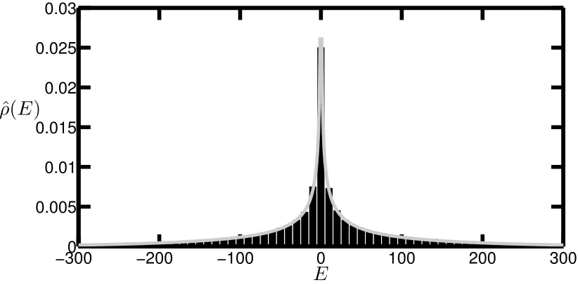
−3000 −200 −100 0 100 200 300 0.005
0.01 0.015 0.02 0.025 0.03
E
[image:8.612.74.485.98.301.2]ˆ
ρ
(
E
)
Figure 2. The grey line represents the analytical result and the histogram shows the numerical data. The numerical simulations were performed over 1000 realizations of random matrices forN = 1000 andσ= 10.
ρ(0) has a maximum value proportional to wi−2. Since negative moments are divergent for the Gaussian distribution, the density of states tends to infinity, if wi are random
Gaussian variables.
Employing the same method one can average the expression for the moments of the eigenvectors (14):
ˆ
Iq ≡ N
X
n
hIq(n)i=
NhsiqΓ(q+ 1) (πρˆ(E)N)q
x2q
[(E−x2hti)2 +hsi2x4]q
x
= E
qΓ(q+ 1)
2qhtiqNq−1
x2q
[(E−x2hti)2+hsi2x4]q
x
.
(24)
The calculation of the averaging over wi can be simplified first by noticing that
x2q
[(E−x2hti)2+hsi2x4]q =
1 (q−1)!
"
− 1 2y
d dy
q−1
x4−2q
(E−x2hti)2 +y2x4
#
y=hsi
, (25)
therefore the averaged moments of the eigenvectors can be written as
ˆ
Iq =
qEq
2qhtiqNq−1
"
− 1 2y
d dy
q−1
x4−2q
(E−x2hti)2+y2x4
x
#
y=hsi
. (26)
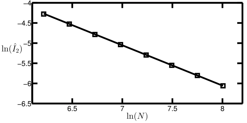
6.5 7 7.5 8 −6.5
−6 −5.5 −5 −4.5 −4
[image:9.612.77.482.99.301.2]ln(
N
)
ln( ˆ
I
2)
Figure 3. The numerical results are given by the symbols and the solid line depicts our analytical result. In this numerical simulation over 1000 realizations of random matrices, we usedσ= 10.
the averaging is completed, we arrive at the final result for the moments
ˆ
Iq =
q√E
2qhtiqNq−1
− 1 2y
d dy
q−1
1
σy
r
π
8
(hti+ iy)q−1F−(hti,hsi)
+ (hti −iy)q−1F+(hti,hsi)
y=hsi
.
(27)
The derivatives can be calculated explicitly for any integer q. Since the final expressions for ˆIq become quite lengthy for higher values of q, here we present only
an explicit formula for q= 2:
ˆ
I2 =
√
E
8Nhti2hsi2σ
r
π
2
"
hti −ihsi hsi +
i 2
1 + E(hti+ ihsi) (hti2+hsi2)σ2
F+(hti,hsi)
h
ti+ ihsi hsi −
i 2
1 + E(hti −ihsi) (hti2+hsi2)σ2
F−(hti,hsi) +
√ 2Ehti √
πσ(hti2+hsi2)
#
.
(28)
In order to corroborate the validity of this expression we ran numerical simulations for
σ = 10. The numerical results presented in Fig. 3 along with the analytical solution fully confirm its validity. The moment with q = 2 was calculated for the eigenvectors corresponding the eigenvalues from the vicinity ofE = 1.
According to Eq.(27) the scaling of ˆIq ∝ N1−q is exactly the same as in GUE,
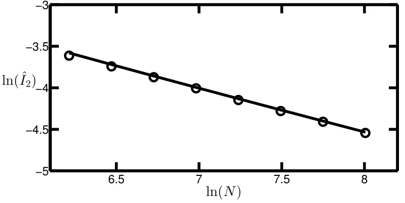
6.5 7 7.5 8 −5
−4.5 −4 −3.5 −3
[image:10.612.80.482.99.301.2]ln(
N
)
ln( ˆ
I
2)
Figure 4. This figure shows the results of numerical simulations (symbols) for ˆI2 at
σ=N1/2. The solid line represents our analytical result. The numerical simulations
were performed over 1000 realizations of random matrices.
conclusion can’t be drawn any more. To explore such a possibility, we study the model with σ =Nγ, γ >0.
Since σ → ∞, as N → ∞ we can analyse the asymptotic behaviour of the simultaneous equations when σ → ∞, assuming that E ∝ O(1), so we set E = 1 for simplicity. One can show that in this limit hsi hti, therefore we can expand all the expression in hti/hsi and keep only the leading order terms. Then the asymptotic solution of the simultaneous equations is given by
hti ≈ √
π
4σ , hsi ≈1. (29)
Substituting this result into the formula for ˆIq we find an asymptotic expression for the
moments:
ˆ
Iq ≈q
σ
√
πN
q−1q−2 Y
k=0
q− 5 + 4k 2
(30)
This result holds for anyσ1. In particular, forσ=Nγwe have ˆIq∝N(γ−1)(q−1). The
scaling of the moments with non-trivial power ofN implies that the eigenvectors become fractal in this case with the fractal dimension Dq = 1−γ. There is a clear similarity
between this finding and recent results [14, 9] for non-ergodic states in the Rosenzweig-Porter model [10]. Indeed, our results for σ = const and σ = Nγ show that there is a
require any fine-tuning of parameters of a model, might be important for understanding of emergence of such states in various applications such as, for example, critical wave functions of certain biomolecules, reported recently in Ref. [15].
We computed ˆI2 numerically for σ =N1/2 for the eigenvectors, whose eigenvalues
are sufficiently close to E = 1, and found the the numerical results are in agreement with our prediction. The corresponding results are given in Fig. 4.
4. Conclusions
We studied a general class of the structured random matrices given by Eq.(1). Our main focus was on the statistical properties of the eigenvectors of such random matrices. Using the supersymmetry technique we derived a very general expression for the local moments of the eigenvectors. This result allowed us not only to make predictions about qualitative nature of the eigenvectors, such as a degree of their ergodicity, but also to understand, how particular components of the eigenvectors are affected by the corresponding matrix elements of W and D.
We investigated in detail a special case of the model with D = 0 and Gaussian distributed W. We found that when the variance of wi scales in a power-law fashion
with N, the eigenvectors of the model become critical and are characterized by a non-trivial fractal dimension, making such ensemble of random matrices to be similar to the Rosenzweig-Porter model.
It would be interesting to generalize our results to other random matrix ensembles. Particularly, in many applications instead of the matrix ˜H from the GUE one should deal with matrices from the Gaussian Orthogonal Ensemble or Wishart matrices.
KT acknowledges support from the Engineering and Physical Sciences Research Council [grant number EP/M5065881/1].
Appendix A. Pre-exponential factors in Efetov’s parametrization
The pre-exponential factors calculated by employing Efetov’s parametrization are given as follows:
gaaBB = E−dn−w
2
nt+ iswn2λ1+ iswn2(λ1−λ2)αα∗
(E−dn−wn2t)2+s2wn4
, (A.1)
garBB = −
µ1sw2n
1 + αα
∗
2 1−
ββ∗
2
+µ∗2sw2
nα
∗β
(E−dn−wn2t)2+s2w4n
, (A.2)
graBB = −
µ∗1sw2
n
1− ββ
∗
2 1 +
αα∗
2
+µ2sw2nβ
∗α
(E−dn−wn2t)2+s2w4n
, (A.3)
grrBB = E−dn−w
2
nt−isw2nλ1+ isw2n(λ1−λ2)ββ∗
(E−dn−w2nt)2 +s2wn4
The integration measure reads
dµ(T) = − dλ1dλ2 (λ1−λ2)2
dφ1dφ2dαdα∗dβdβ∗, (A.5)
where λ1 ∈ [1,∞), λ2 ∈ [−1,1], φ2, φ2 ∈ [0,2π], and α, α∗, β, β∗ are Grassmann
variables, for which the following convention is used
Z
dα α=
Z
dα∗ α∗ =
Z
dβ β=
Z
dβ∗ β∗ = √1
2π. (A.6)
Appendix B. Computing the average in Eq.(19)
The integral over x can be computed by the application of the residue theorem, which gives
Z ∞
−∞
dx (2Ex
2hti −E2)e−iκx
x2− Ehti
hti2+hsi2
2
+ E2hsi2 (hti2+hsi2)2
= π hti
2
+hsi2√
E
2hsi
× phti −ihsi hti+ ihsie
−i|κ|qhti+iEhsi
+phti+ ihsi hti −ihsie
i|κ|qhti−hEsi !
,
(B.1)
where we made the following assumptions: E >0, hti>0 and hsi>0. Therefore the average is equal to
*
2Ex2−E2
x2− Ehti
hti2+hsi2 2
+ E2hsi2 (hti2+hsi2)2
+
x
= √1 2π
Z ∞
−∞
dκ√1 2πe
−1 2κ
2σ2π hti
2
+hsi2√
E
2hsi
× phti −ihsi hti+ ihsie
−i|κ|q E
hti+ihsi + hti+ ihsi
p
hti −ihsie
i|κ|q E
hti−hsi
!
,
(B.2) computing the integral over κwe arrive at the result
*
2Ex2−E2
x2− Ehti
hti2+hsi2 2
+ E2hsi2 (hti2+hsi2)2
+
x
= 1
hti2+hsi2
× 1 + √ E
2hsi
r
π
2
e−
Ehti
(hti2+hsi2)σ2
q
hti2+hsi2σ
e
E
2(hti−ihsi)σ2(hti −ihsi)3/2
× 1−erf
"s
− E 2(hti+ ihsi)σ2
#!
+e
E
2(hti+ihsi)σ2(hti+ ihsi)3/2 1−erf
"s
− E 2(hti −ihsi)σ2
where erf is the error function. The expression above can be simplified down to
1 = 1
hti2+hsi2
1 +
√
E
2hsi
r
π
2
e−
Ehti
(hti2+hsi2)σ2
q
hti2+hsi2σ
e
E
2(hti−ihsi)σ2(hti −ihsi)3/2
× 1−ierfi
"s
E
2(hti+ ihsi)σ2
#!
+e
E
2(hti+ihsi)σ2(hti+ ihsi)3/2
× 1 + ierfi
"s
E
2(hti −ihsi)σ2
#!
.
(B.4)
In the integral for the moments we are then able to compute the average by applying the Fourier transform and integrating over the expressions
1 hti2+y2
*
(x2)2−q
x2− Ehti
hti2+y2
2
+ E2y2
(hti2+y2)2
+
x
= √1 2π
Z ∞
−∞
dκ√1 2πe
−1 2κ
2σ2
1 hti2+y2
Z ∞
−∞
dx (x
2)2−qe−iκx
x2− Ehti
hti2+y2
2
+ E2y2
(hti2+y2)2
.
(B.5)
Once the integral over xhas been completed we arrive at the following
1 hti2+y2
*
(x2)2−q
x2− Ehti
hti2+y2
2
+ E2y2
(hti2+y2)2
+
x
= E 1 2−q 2y
Z ∞
0
dκe−12κ 2σ2
(hti+ iy)q−32e−iκ
q
E
hti+iy + (hti −iy)q−32eiκ
q
E
hti−iy
!
,
(B.6)
the integral over κ can also be calculated, which yields the final expression for the moments averaged over wi, this is valid for any integer q
ˆ
Iq =
q√E
2qhtiqNq−1
− 1 2y d dy
q−1
1 σy r π 8 e− E
2(hti+iy)σ2(hti+ iy)q−32
1−ierfi "s
E
2(hti+ iy)σ2
#
+e
− E
2(hti−iy)σ2(hti −iy)q−32
1 + ierfi "s
E
2(hti −iy)σ2
#
y=hsi
.
(B.7)
References
[2] R. Nadakuditi and A. Edelman, IEEE Trans. Signal Process.56, 2625 (2008). [3] C. Soize, Journal of Sound and Vibration 263, 893 (2003).
[4] R. Couillet and M. Debbah, Random matrix methods for wireless communications, (Cambridge University Press, 2011).
[5] Y. Ahmadian, F. Fumarola, and K. D. Miller, Phys. Rev. E91, 012820 (2015). [6] J. Grela and T. Guhr, Phys. Rev. E94, 042130 (2016).
[7] P. Bourgade and H.-T. Yau, Commun. Math. Phys. 350, 231 (2017). [8] K. Truong and A. Ossipov, J. Phys A: Math Theor49, 145005 (2016). [9] K. Truong and A. Ossipov, Europhys. Lett. 11637002 (2016).
[10] N. Rosenzweig and C. E. Porter, Phys. Rev.120, 1698 (1960). [11] A. D. Mirlin, Phys. Rep.326, 259 (1999).
[12] F. Haake,Quantum Signatures of Chaos, (Springer, 2001). [13] Y. V. Fyodorov, J. Phys. A.32, 7429 (1999).
[14] V. E. Kravtsov, I. M. Khaymovich, E. Cuevas, and M. Amini, New Journal of Physics17, 122002 (2015).