Non parametric representation and prediction of single and multi shell diffusion weighted MRI data using Gaussian processes

Non-parametric representation and prediction of single- and multi-shell

diffusion-weighted MRI data using Gaussian processes

Jesper L.R. Andersson

⁎

, Stamatios N. Sotiropoulos

FMRIB Centre, University of Oxford, UK

a b s t r a c t

a r t i c l e i n f o

Article history: Received 11 March 2015 Accepted 26 July 2015 Available online 30 July 2015 Keywords:

Diffusion MRI Gaussian process

Non-parametric representation Multi-shell

Diffusion MRI offers great potential in studying the human brain microstructure and connectivity. However, dif-fusion images are marred by technical problems, such as image distortions and spurious signal loss. Correcting for these problems is non-trivial and relies on having a mechanism that predicts what to expect. In this paper we de-scribe a novel way to represent and make predictions about diffusion MRI data. It is based on a Gaussian process on one or several spheres similar to the Geostatistical method of“Kriging”. We present a choice of covariance function that allows us to accurately predict the signal even from voxels with complexfibre patterns. For multi-shell data (multiple non-zerob-values) the covariance function extends across the shells which means that data from one shell is used when making predictions for another shell.

© 2015 The Authors. Published by Elsevier Inc. This is an open access article under the CC BY license (http://creativecommons.org/licenses/by/4.0/).

Introduction

Diffusion weighted MR imaging makes it possible to map the micro-structure and the connectivity of the living human brain. It proceeds by acquiring a set of echo planar images (EPI), each with the signal spoiled by a gradient such that the signal is lower in areas/voxels where water diffuses freely in the direction of that gradient. By acquiring many such images it is possible to build a pro_file of diffusivity in_“any_” direc-tion for each voxel which can subsequently be used to probe the under-lying microstructure and estimate white matter tracts by following the path of greatest diffusivity.

However, diffusion imaging is also marred by technical problems such as image distortions, subject movement and spurious signal loss caused by macroscopic movement during the diffusion encoding. Correcting for distortions and movement is a non-trivial problem since the distortions depend on the diffusion gradient and hence are different for each volume (see for exampleAndersson and Skare, 2002orRohde et al., 2004). Image registration based solutions are dif_ficult since each volume will also have a different contrast and often (when applying strong diffusion weighting) poor SNR. The spurious signal loss will typi-cally affect a whole, or a substantial part of a, slice but can be dif_ficult to detect. It entails detecting a“smaller than expected”signal in a slice, but that hinges on knowing what to expect, which is non-trivial.

This paper describes a new way to model and predict diffusion signal from MR experiments. Unlike parametric models (Panagiotaki et al. (2012)) like for example the diffusion tensor (Basser et al. (1994)) or the ball-and-stick model (Behrens et al. (2003)), the model we propose

will not yield biologically relevant parameters that are of value in their own right. Instead it is only used for making predictions about observed or unobserved measurements, which is something we will utilise in two related papers for:

• Correcting for distortions and subject movement by alignment of an observed volume to a predicted volume.

• Detection and replacement of outliers, typically signal loss caused by coherent movement during the diffusion encoding.

The representation we propose to use to describe the diffusion signal is a Gaussian process (GP). We should note that short preliminary de-scriptions of the distortion correction application of the Gaussian pro-cess predictor have been given in Andersson et al. (2012) and

Sotiropoulos et al. (2013)and of its application to outlier detection in

Andersson and Sotiropoulos (2014). The predictor forms the backbone of many of the preprocessing steps of the state-of-the-art data collected in the Human Connectome Project (Van Essen et al. (2013)). In this paper we describe in detail the underlying theory of theGPpredictor and illustrate its working principles.

Theory

Gaussian processes

Introduction to Gaussian processes

Let us say we have a stochastic variableYthat is distributed as

Y Nμ;σ2 _ð1Þ

⁎ Corresponding author at: FMRIB Centre, JR Hospital, Headington, Oxford OX3 9DU, UK. E-mail address:[email protected](J.L.R. Andersson).

http://dx.doi.org/10.1016/j.neuroimage.2015.07.067

1053-8119/© 2015 The Authors. Published by Elsevier Inc. This is an open access article under the CC BY license (http://creativecommons.org/licenses/by/4.0/).

Contents lists available atScienceDirect

NeuroImage

i.e.has a Gaussian distribution. This means that if we were to take an ob-servationyfromY, we would expect to see a value“not too far off”μand if we were to make a series of observations we would expect 68% of those to fall in the range [μ−σ,μ+σ].

A Gaussian process extends the concept of a stochastic variable to a stochastic function. Analogously to the stochastic variable above, we can say that a stochastic functionf(x) is distributed as

f xð Þ GPðm xð Þ;k xð ;x0ÞÞ ð2Þ

i.e.as a Gaussian process (Rasmussen and Williams (2006)) with a mean functionm(x) and a covariance functionk(x,x′). To understand Gaussian processes it can be useful to consider ap-dimensional stochas-tic variable distributed as

Y Npðμ;ΣÞ ð3Þ

i.e.according to a multivariate normal (MVN) distribution characterised by ap× 1 mean vectorμand ap×pcovariance matrixΣ. If we were to take a sampleyfromYwe would now expectyto be“close”toμ, and if we were to take many samples we would expect most of them to fall within the confidence contours given byΣ. The role ofΣin this context is to describe how variable the different elements ofYare,andalso how they covary. If for exampleΣ12has a large positive value it is less sur-prising if bothy1andy2have a value larger thanμ1andμ2(or smaller) than if one of them is larger and the other smaller.

Analogously one could take a sample fromf(x) and we would expect that sample to be“close”to the mean functionm(x). And how surprising we wouldfind deviations fromm(x) depends onk(x,x′). In contrast to the MVN case this sample is a continuous function,i.e.it has a value for eachx, though it may not have any parametric form. Another impor-tant distinction is thatk(x,x′) is a continuous function with a value for any pair (x,x′) ofx-values. Also, becausexis a continuous variable it is meaningful to define a distance between two pointsxandx′, unlike the case of the elements ofywherey1andy2could represent complete-ly different entities.

Just as most applications of Gaussian distributions are inverse prob-lems, where given a sampleyone wants tofind estimates forμandσ2_, most applications of Gaussian processes aim to estimate the mean func-tionm(x) given some set of observed pairs (xi,fi) (often called the “training data”or the“training set”). The next section will explain how that is achieved.

Making predictions (estimating m(x))

For this section we will assume that there is a covariance function k(x,x′) that is known to us. How we actuallyfindk(x,x′) will be the sub-ject of the next section.

As stated above,m(x) may not have a parametric form, and even if it did it is not known to us. Given that, how can a continuous function onx, i.e.one where for any arbitrary valuexwe can calculate a valuef(x), be meaningfully described? To answer that wefirst reorganise the training data into a vector ofnobservations of the independent variable which we callxand a vector of observations of the function (dependent variable) that we callf. We can then write the joint probability of the training data and any (unobserved) pair (x*,f*) as

f

f Nnþ1 0; K xð ;xÞ k x;x

ð Þ

kðx;xÞ k xð ;xÞ

ð4Þ

whereK(x,x) is ann×nmatrix of covariances between all the points in the training data,k(x,x*) is ann× 1 vector of covariances between the unobserved pointx* and the training data and wherek(x*,x*) is simply the variance at the pointx*. It may seem counter intuitive that the MVN above has a zero mean, but that only means thatf(x) is assumed to have a zero mean when averaged over allx. Typically one just subtracts the

mean (f) fromfand then add it back tof*, which is analogous to what is often done in“traditional”regression.

In Eq.(4)everything is known exceptf* so in order to maximise the joint probability we just need to maximise the probability off* condi-tional onx*,xandfwhich can be expressed as

p fð jx;x;fÞ ¼ N ðkðx;xÞK x;ð xÞ−1_f;

k xð ;xÞ−kðx;xÞK x;xÞ−1_{k x;}

x

ð Þ

ð5Þ

and the value off* that maximises it is of course the expectation k(x*,x)K(x,x)−1_{f. This is similar to the E-step of the EM algorithm} (Dempster et al., 1977) for MVN data with missing observations.

The estimation given by Eq.(5)assumes that the training data is “perfect”,i.e.that there is no uncertainty in the observationsfof the dependent variable. The covariance functionk(x,x′) doesnotmodel any error in the data, but the variability of the function itself. If we were to calculatek(x*,x)K(x,x)−1_ffor

“all_”values ofx* we would see that the resulting plot passed exactly through all of the training points (xi,fi).

Hence, in order to be able to use this with our data, which are always noisy, we need to complement it with a model for the measurement error. This means that Eq.(4)changes to

f

f Nnþ1 0;

K xð ;xÞ þσ2_{I k xð ;xÞ} kðx;xÞ k xð ;xÞ

ð6Þ

and the conditional expectation and variance change to

^f xð Þ ¼ kðx;xÞK xð ;xÞ þσ2_I−1_{f ð7Þ}

and

Cov^f xð Þ ¼k xð;xÞ−kðx;xÞK xð ;xÞ þσ2

I

−1

k xð ;xÞ ð8Þ

respectively, whereσ2

is the variance of the observation error (it will be explained later how we estimateσ2_{) and whereIis then×nidentity} matrix.

Eq.(7)provides a way to make predictions for both observed and unobserved pointsx* given some observationsxandf,providedthat we know the functionk(x,x′).

Finding k(x, x_′)

There are a lot of suggestions for covariance functionsk(x,x′) in the literature about Gaussian processes. They are typically devised so that nearby points have a larger positive covariance than points further apart thereby imposing smoothness on the function. For a function k(x,x′) to work as a covariance function it needs to produce a positive definite matrixK(x,x) for any setxof points in the domain off(x) (seee.g.Genton, 2001).

Many existing covariance functions, such as for example the squared-exponential (Rasmussen and Williams, 2006), are parametric, i.e. they have a number of free parameters (often referred to as hyperparameters) whose values determine the detailed properties of the resultingGP. The task offinding a suitable covariance function for one's application/data entails not only choosing the“right”parametric form but also, possibly on a per data set basis, suitable values for the pa-rameters. This can be achieved by marginal likelihood maximisation (Rasmussen and Williams, 2006), or by leave-one-out methods (Sundararajan and Sathiya Keerthi, 2001).

Gaussian processes for diffusion data

This section builds the case for the covariance functions we suggest for diffusion data.

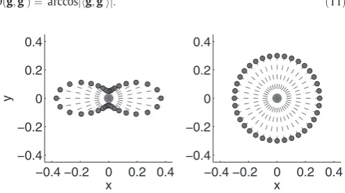
the data can be seen as a response variable (the signal) acquired on the surface of a sphere. The weighting is typically characterised by ab-value that speci_fies the strength of diffusion weighting and a unit length vec-torgthat specifies the direction. The signal is affected by the local diffu-sion of water molecules such that a high diffusivity alonggleads to a small signal. A full diffusion protocol consists of multiple measurements along different directions aimed at characterising the diffusion along “any”direction. A two-dimensional demonstration of how the diffusion signal might look can be seen inFig. 1. This shows two important as-pects of the diffusion signal:

• The signal changes smoothly as the angle of the diffusion weighting direction changes.

• The signal is axially symmetric,i.e.the signal alonggis identical to the signal along−g.

Because the diffusion signal lives on a sphere, it is a good match for techniques that have been developed and used for geostatistics and me-teorology where a special case ofGPs observed on a sphere is known as “Kriging”(Wackernagel, 2003). For these techniques the covariance is often defined as a function of an angleθbetween two vectors from the centre of the sphere toxandx′. These vectors are easily recognised as theg-vectors described above. Two popular covariance functions in geostatistics are the“Exponential model”

Cð Þ ¼θ e−θ=a _{for 0≤θ≤π ð9Þ}

whereais a positive scale parameter, and the_“Spherical model_”where ais again a positive scale parameter that here determines the“distance” at whichθthe covariance goes to zero:

Cð Þ ¼θ 1−3_2aθþ θ 3

2a3 if θ≤a

0 if _θNa

8 <

: : ð10Þ

Both of these are“valid”covariance functions (Huang et al., 2011) on the sphere,i.e.they will yield invertible matricesKand the marginal likelihood will exist for any data. For diffusion data we need to modify the definition ofθsince we want the model to be symmetrical on the sphere. We do this by definingθfor two unity length diffusion gradient vectorsgandg′as

θðg;g0Þ ¼arccosjhg;g0ij: ð11Þ

This is equivalent to extending both vectors also in the negative direction and choosing the smallest of the two angles between the resulting crossing lines.

Single shell data

When all the diffusion weighted measurements are performed with the sameb-value, data are said to be collected on a single shell, which is then very similar to the geostatistical application of Kriging. One can ob-tain an idea about the form of the covariance function by calculating a sample covariance and plotting the elements of that matrix againstθ. The resulting plot can be seen inFig. 2, and both the exponential and the spherical covariance functions capture the general appearance of the observed covariance, with the spherical model possibly looking a little better. To estimate the optimal hyperparameters for each model one can use marginal likelihood maximisation (also known as type II maximum likelihood) (Rasmussen and Williams, 2006) which maximises

logpðyjβ;MÞ ¼−1₂yT_K−1 y y−

1

2logKy þc ð12Þ

whereyis the signal from one voxel for all the diffusion directions, where

β= [λaσ2_{] and whereK}

y=K+σ2IandKis the matrix with elements Kij=λC(θij;a) whereC(θ;a) is given by Eq.(9) or (10)depending on which modelMis being considered. In these models,ais a“distance scale”parameter determining how fast the covariance decreases as one moves along the surface of the sphere,λis a“signal scale” pa-rameter which determines the variability of the signal andσ2

deter-mines the uncertainty of the measured valuesy. When estimating the hyperparameters the model was reparameterised so that~_λ¼eλ

andσf2_¼eσ2

were estimated rather thanλandσ2

themselves so as to avoid the possibility of negative scaling or variance.

The term“marginal likelihood”seems a little counter intuitive since it is not immediately clear what is being marginalised over.“Normally” when estimating the values of some hyperparameters the marginalisation occurs over the lower level parameters of the model. In the case of Gaussian processes the“parameters”are all possible functionsf(x) and we recommend chapters 2 and 5 ofRasmussen and Williams (2006)for an explanation of this.

When maximising Eq.(12)onefinds the optimal hyperparametersβ

for the particular voxel from whichyis taken. However one would like tofind a singleβfor all voxels. Tofind that, Eq.(12)is summed over all (or at least a sizeable subset of all) voxels, which is equivalent to multi-plying the likelihoods over voxels (Minka and Picard, 1999).

Eq.(12)still cannot be used to choose between the models. For that we would need the model evidence

pðMijyÞ∝pðyjMiÞ ¼Z

βpðyjβ;MiÞpðβjMiÞdβ ð13Þ

wherep(β|Mi) is the prior distribution ofβ. In order to calculate the in-tegral in Eq.(13)we use Laplace's approximation which entailsfinding theβwhich maximisesp(y|β,Mi), calculating the Hessian at that point

β0and approximatingp(β|Mi) by a Gaussian distribution centred onβ0 and the covariance given by the inverse Hessian. We leave the details of those calculations toAppendices A and B.

It is true that Laplace's equation is an approximation, but it should be noted that the ability of a Gaussian process to make useful predictions (i.e.to estimate the mean function through Eq.(7)) is not strongly dependent on the exact form of the covariance function (Press et al., 2007).

Leave-one-out methods

In addition to the marginal likelihood maximisation we also im-plemented and tested methods based on maximising the ability to predict unobserved data. In the interest of space we will not present

−0.4 −0.2

0

0.2 0.4

−0.4

−0.2

0

0.2

0.4

y

x

−0.4 −0.2

0

0.2 0.4

−0.4

−0.2

0

0.2

0.4

x

Fig. 1.Simulated (2D) examples of diffusion weighted measurements. The direction along which diffusion weighting was applied is shown by a dashed line and the measured signal along that direction is indicated by the distance of the round marker from the origin. The left panel shows the case where diffusivity is three times greater along they-axis than along thex-axis. The right panel demonstrates the case where diffusivity is equal in all di-rections. The extension of this to 3D is straightforward, though a little tricky to demon-strate in afigure. If we extend thefigure in the left panel to 3D and assume that the diffusivity along the direction perpendicular to the paper is the same as for the x-direction, the points sampled on the resulting surface would form a“red blood cell”

any results derived with those methods and simply mention that we implemented and tested the methods referred to as Cross-Validation (CV), Geisser's Surrogate Predictive Probability (GPP) and Geisser's Predictive mean Square Error (GPE) as described inSundararajan and Sathiya Keerthi (2001). We found that both CV and GPP yielded hyperparameters that obtained good predictions and hence they are both part of our implementation. In contrast toSundararajan and Sathiya Keerthi (2001)we found that GPE did not perform well.

Multi-shell data

Increasingly diffusion data is acquired with two or more different non-zerob-values (see for exampleAlexander et al., 2006;Aganj et al., 2010;Sotiropoulos et al., 2013orSetsompop et al., 2013). This type of data is referred to as“multi-shell”data. The logic behind this name is that the data collected for eachb-value forms a closed 2D surface em-bedded in 3D space where the surface resulting from the highb-value is completely enclosed inside the surface formed by the lowb-value. The rational behind such an acquisition is that highb-values give more angular contrast and higher“diffusion resolution”but lower SNR than lowb-values.

A general strategy for defining covariance functions is to construct new functions from products or linear combinations of existing ones (Rasmussen and Williams, 2006). For multi-shell data two points may differ on two axesθandΔbwhereθis defined as above andΔbis the difference inb-value between the two points. A“natural”covariance function for multi-shell data would hence be

kðx;x0Þ ¼Cθðθðg;g0Þ;aÞCb b−b0;ℓ

ð14Þ

whereCθis the covariance function we defined above for the single shell

case, whereCbis some candidate smooth function describing how the covariance changes along thebdirection and whereℓis some set of hyperparameters forCb.

We have chosen the squared-exponential (Rasmussen and Williams, 2006) covariance function forCband have used the log of theb-values as the measure of distance along theb-direction. Hence,Cbis given by

Cb b;b0;ℓ

¼ exp − logb−logb0

2

2ℓ2 !

: ð15Þ

Multi-shell acquisition schemes typically consists of a smallfinite set (often 2–3) of shells in thebdirection. For each of those shells we allow for a unique measurement error. If we assume that we have two shells, the fullK-matrix can be written as

K¼ λCθðθð Þ;G1 aÞ þσ 2

1I λCθðθðG2;G1Þ;aÞCb b2;b1;ℓ

λC_θðθðG1;G2Þ;aÞCb b1;b2;ℓ

λC_θðθð Þ;G2 aÞ þσ22I

2 4

3 5

ð16Þ

where the hyperparameters that need to be estimated areβ= [λaℓσ12

σ22], whereθ(G,G′) is a matrix-valued function with all the angles between theg-vectors in the setsGandG′, whereCθ is given by

Eq.(9) or (10)and whereCbis given by Eq.(15). Eq.(16)is trivially extended to theN-shell case and the number of hyperparameters goes as 3 +N.

The same marginal likelihood maximisation that was described for the single shell case can be used to determine the hyperparameters of the multi shell case, as can either of the prediction based methods referred to inSection 2.2.2.

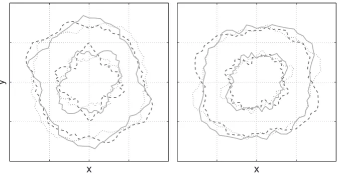
InFig. 3we demonstrate the“Prior shapes”given by the single-(left panel) and multi-shell (right panel) models. A prior shape is a shape that has been drawn from the distribution of plausible shapes given the form of the covariance function and the values of the hyperparameters. Any shape has a probability of being drawn that is proportional to its prior probability (i.e.in the absence of any data). It can be seen that the prior favours approximately spherical shapes in the absence of any evidence to the contrary.

A note on optimisation

It is suggested, for example inRasmussen and Williams (2006), that an optimisation method that uses derivative information should be used whenfinding the hyperparameters that maximise Eq.(12). The reason for that is that such methods typically use fewer steps, and when the cost of calculating the derivatives is small/moderate com-pared to calculating the functions itself (as is the case for Eq.(12)) then execution time can be much shorter. However, we found that for the multi-shell case a heuristic optimisation method such as the Nelder–Mead simplex method (Nelder and Mead, 1965) was frequently better at avoiding local maxima. Hence, that was the method we used for all optimisations in the present paper.

0 pi/8 pi/4 3pi/8 pi/2

−1 0 1 2

b=3000

Angular distance

Covariance (arbitrary scaling)

0 pi/8 pi/4 3pi/8 pi/2

−1 0 1 2

b=7000

Angular distance

Covariance (arbitrary scaling)

Materials and methods

3.1. Diffusion data

In order to ensure that results are not specific to a particular scanner and/or protocol, data was taken from several studies performed by several groups. The common feature of all data sets is that they are at the upper end of what is usually acquired in terms of number of directions andb-values. Relevant key parameters are summarised inTable 1.

After acquisition, data was corrected for susceptibility induced distortions (in the case where data was acquired with reversed phase-encode directions) and eddy current induced distortions and subject movement. It may seem circular that we used our Gaussian process based method for distortions and movement to correct the data prior to using it in the present paper. How this is performed is briefly ex-plained inAppendix C.

Analysis

Single shell model selection

For each of the data sets three slices through the centre of the brain were selected and all the intra cerebral voxels of those slices were used. The hyperparameters for both models (given by Eqs.(9) and (10)) were estimated by maximising the log marginal likelihood (Eq. (12)) summed over all voxels. The evidence was calculated for each model as described inAppendices A and Band for each data set, the Bayes fac-tor comparing the two models was calculated.

Predictions

The model selected based on the previous section was used to make predictions of diffusion weighted volumes. Predictions were made both including the observed data for the predicted volume (in which case theGPperforms a smoothing on the sphere) and ex-cluding it (in which case theGPcorresponds to an interpolation) in the training data.

In order to see how the model allows us to improve predictions for one shell by utilising information from other shells we subsam-pled one of the shells and calculated predictions for that shell in iso-lation (Eq.(9) or (10)) and in the context of one or more other shells (Eq.(16)).

Results

Single shell model selection

All data sets showed a very strong preference for the spherical model (Eq.(10)) over the exponential model (Eq.(9)). Even for single voxels, the Bayes factor (Kass and Raftery (1995)) ranged from 1 (for voxels in CSF) to_N10,000 (white matter voxels with strongest preference). When estimating a single set of hyperparameters from a large selec-tion (N10,000) of intracerebral voxels, the resulting Bayes factor was so large that it approached the numerical precision of a double. This finding was independent of the data set used. It was therefore decided to use the spherical model for all further analysis.

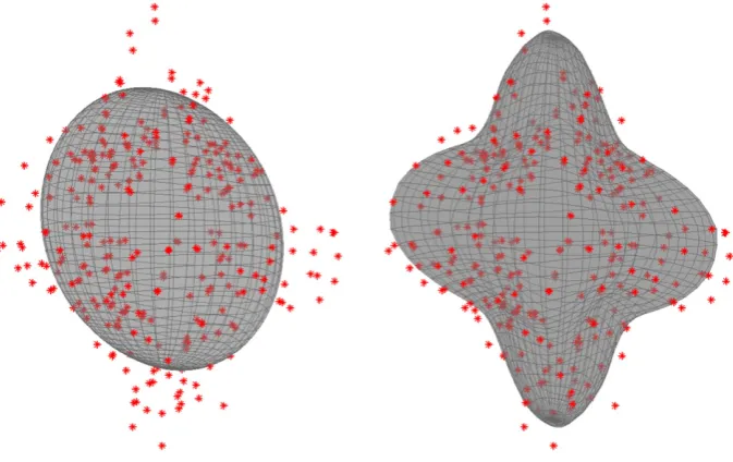
Fig. 4shows the predictions made by the tensor model and the suggestedGP. The data inFig. 4comes from a white matter voxel with a three-way crossing (each local minimum on the modelfit in the right panel represents afibre direction). It can be seen that the Gaussian process is able to model the structure of the signal very well without any obvious“overfitting”.

InFig. 5we demonstrate the impact of the hyperparameters on the ability of theGPto model the data. It shows data from two voxels, one in grey matter and one from a white matter region with complex architecture (i.e.crossingfibres). Three sets of hyperparameters are es-timated, from the grey matter voxel, from the white matter voxel and jointly from both. All three sets of hyperparameters are subsequently used to model data from both voxels. It can be seen that both the hyperparameters estimated from the white matter and those estimated from both yields processes that are able to adequately model either voxel.

x

y

x

Fig. 3.Examples of prior shapes (cut at arbitrary plane) generated using hyperparameters estimated from the HCP b = 1500 data (outer shell) and the HCP b = 5000 (inner shell). The solid, dashed and dotted shapes represent three different realisations drawn from the distribution of possible shapes. On the left hand side the priors were drawn independently for the two shells and on the right they were drawn from the multi-shell model (Eq.(16)). Note how in the absence of data, the expected shape is approximately spherical (isotropic diffusion) and that the (relative) variability is greater for the inner shell. Note also that for the multi-shell model (right hand size) the shapes covary across the shells.

Table 1

The table shows a few key parameters for the data that was used for testing theGP. RP stands for Reversed Polarity and implies that each diffusion gradient was acquired twice with opposing phase-encode directions.

Scanner b-Value # of directions Resolution (mm)

RP Reference

Siemens Verio 1500 120 23

mm3

Yes Siemens Trio 2500 124 2.23

mm3

No 1500

3000

Siemens Skyra 5000 300 23_mm3 _{Yes Uğurbil et al. (2013)}

7000

MGH-HCP 10,000 198 1.53

mm3

The Gaussian process is able to model highb-value data from voxels with vastly different signal profiles. To show that, we estimated hyperparameters from a random selection of 1000 intracerebral voxels in a data set acquired with ab-value of 7000. The resulting Gaussian process was used to model data from six randomly selected voxels from a plane at the level of the crossing of the superior longitudinal fas-ciculus II and the cortico spinal tract. The results are shown inFig. 6.

Multi-shell model

Fig. 7shows data and the resulting predictions for two shells withb -values 1500 and 5000 when using model(16). The prediction at any point (any point on either of the surfaces) is a linear combination of the data points with higher weights given to the points with similarθandϕ

(in spherical coordinates) and higher weights to points on the same shell. Fig. 4.Example of predictions from a tensorfit (left) panel and from a Gaussian processfit (right) panel to a crossingfibre voxel in the Centrum Semiovale in the region where the superior longitudinal fasciculus II crosses the corticospinal tract. The data is a single shell with ab-value of 3000. The data is shown as red dots and the model prediction as a grey surface. As expected the Gaussian process shows a much better ability to predict the data from such voxels despite being even faster to calculate than the tensor prediction.

The ability to improve the predictions for one shell by utilising infor-mation from (an)other shell(s) is demonstrated inFig. 8.

Predictions

Fig. 9demonstrates that the model was capable of making very accu-rate predictions both when including and excluding the observed data corresponding to the prediction.

Discussion

We have demonstrated the use of Gaussian processes for model-ling and making predictions about diffusion data. For each new

data set a small number (three for most acquisition protocols) of hyperparameters have to be non-linearly estimated and following that all voxels can be modelled using a fast linear method. Despite its speed and simplicity it can model voxels with several crossingfibres.

Gaussian processes are sometimes touted as“model free”, and therefore as a solution to the problem where one has some data that one wants to model but one doesn't have a good theoretical argument for choosing one model over another. This is partially true, but when using Gaussian processes the task has shifted fromfinding a parametric model for the function tofinding a parametric model for the covariance functionk(x,x′).

It may seem counterintuitive that a Gaussian process with a single set of hyperparameters (estimated from voxels that represent a mixture Fig. 6.Thefigure shows data (red) and Gaussian process (GP)fit (grey) from a b = 7000 shell from the pilot phase of the HCP. The six panels correspond to six randomly selected voxels in a transversal slice at the level of the Centrum Semiovale. The hyperparameters for theGPwas the same for all voxels (and calculated from a random selection of 1000 intracerebral voxels). It can be seen that theGPhas been able to successfully model the signal from the six voxels despite exhibiting vastly different signal profiles. It can for example be appreciated from the signal that the top panel in the middle column corresponds to a three-way crossingfibre, the top panel in the right column a two-way crossingfibre and the lower panel in the middle column a single (dominating)fibre. The top-left and bottom-right panels correspond to grey matter voxels.

of tissue types) can model highly structured data from crossingfibre white matter (such as shown inFigs. 4 to 8) as well as from grey matter or CSF. To understand that, it should be realised that the covari-ance function acts only as a prior on the shapes that can be modelled by theGP. The estimated hyperparameters will be dominated by the white matter signal, because it is only for white matter that there is apprecia-ble signal variation on the sphere. Even so, the most likely shape before observing any data (prior shape) will be spherical (this is true for all“proper”covariance functions on the sphere) so there will be no problems modelling the grey matter or CSF. At the same time there will be enough signal variability (parametrised byλ) to adequately capture the structure in white matter.

The reason we have opted for a Gaussian process rather than some previously published parameteric model (seePanagiotaki

et al. (2012)for examples of biophysical models) is more pragmatic than for its presumed“model freeness”. A Gaussian process is linear, like the single diffusion tensor model after log-transformation of the data, which means it is practical (i.e. fast) to incorporate into a framework where the model has to be re-estimated several times as part of an iterative procedure. In fact, even for the HCP data where each prediction is an inner product of two 300 × 1 vectors, it is twice as fast to calculate as the tensor-based prediction, and for data sets with less points, the difference becomes greater. At the same time it is not so strictly limited in terms of what it can model as the single tensor model, which means that it can better model the signal in areas with for example crossingfibres. It is also less in-herently sensitive to artefactual signal loss than the log-transformed least-squares tensor model.

Fig. 8.Thisfigure demonstrates the predictions for ab= 5000 voxel when considering only theb= 5000 data points (top row) or when using also theb= 3000 data (middle row) or the b= 1500 data (bottom row). The predictions are shown when using only thefirst 10, 25 and 50 points from a set of 300 as well as when using all 300 points. It can be seen (middle row) that the ability to make meaningful predictions from a paucity of data is very much improved when utilising information from the neighbouring shell (b= 3000). It can also be seen (bottom row) that when the“supporting shell”is further away, its impact is smaller, but still appreciable when the number of data points is 25 or less.

There are other methods for modelling the diffusion signal that are less restrictive than the diffusion tensor and still computationally feasi-ble, such as for example spherical harmonics (Descoteaux et al., 2006) or Watson direction functions (Rathi et al., 2009). Compared to these our approach offers the advantage of not having to decide on an order of harmonics or number of direction functions. It also offers (in common withDescoteaux et al., 2011) the ability to simultaneously model multiple shells with the estimates from one shell informing the others. Furthermore we aim to develop correction techniques that are as independent as possible of how the subsequent processing/ analysis of the data is performed so as to avoid circularities. Hence we wanted to avoid commonly used models such as those mentioned above (Descoteaux et al., 2006orRathi et al., 2009). Apart from the circularity argument it is likely that for example a spherical/solid har-monics model with priors on the parameters to ensure spherical prior shapes could equally work for our purposes.

The way in which the Gaussian process can use information from one shell to aid in the prediction of another shell is through the observed covariances between the shells (which will determine the value of the‘hyperparameter in Eq.(15)). That means that if two shells are far apart, and especially if one of the shells has“low”b-values, the observed covariance will be small and the predictive power of one shell on the other will be small. This can be seen inFig. 8where it is demonstrated that ab= 3000 shell will have a substantial impact on the predictions made for ab= 5000 shell when there is a paucity of data, whereas ab= 1500 shell will have a much smaller, albeit non-zero, impact. It can also be seen that when theb= 5000 shell gets more data the impact of the other shells diminishes as the within-shell covariances starts to dominate.

As outlined in theIntroductionsection we plan to use this model for two purposes, thefirst being correction for eddy current distortions and subject movement. In general it is a dif_ficult and largely unsolved prob-lem how to register images acquired with different diffusion gradients because of their different information contents. At the same time it is often desirable to register them, because long study durations make it likely that the subject will have moved between some of the volumes, and because each volume tend to be distorted in a unique way that is determined by the direction and strength of the diffusion gradients (see for exampleAndersson and Skare (2011)for an overview). Our intended use of the Gaussian process model is to register the observed images to their predictions. Since the predictions are based on all (or a majority ifabπ/2) volumes, the resulting prediction will be closer to the average space of the study both in terms of distortions and subject position, than the corresponding observed image. Hence, by iteratively nudging each volume closer to the corresponding prediction we obtain a registered set of images.

The second planned use for this model is outlier detection and re-placement (briefly described inAndersson and Sotiropoulos, 2014). It is not uncommon for diffusion weighted images to suffer from a loss of signal, that may be quite severe. This is caused by (tiny) subject movement or pulsatile movement of the brain (Pierpaoli, 2011) during the diffusion weighting which causes a translation of the signal in k-space, potentially to partially outside thek-space window that is sam-pled. If uncorrected this signal loss will be interpreted as high diffusivity in the direction of the gradient of the affected volume and will bias tractography. There are methods for detecting such outliers (for exam-ple RESTORE,Chang et al., 2005) but these are all based on one specific model (typically the tensor) for the diffusion signal. Consider for exam-ple the left panel inFig. 4where the lack of modelfit would imply a large number of outliers, but where the real issue is an inadequate model. The suggested Gaussian process in contrast is mainly data driven and inde-pendent of the particular model that is used for the subsequent analysis/ tractography. It should be noted that moreflexible models have been suggested for outlier detection (see for examplePannek et al., 2012) and that they would not suffer from the problems that the tensor model does.

Conclusion

We have suggested a method for modelling the diffusion sig-nal that enables us to make accurate predictions. It is based on a Gaussian process, is highly data driven and allows for multi-shell modelling.

Acknowledgments

The authors would like to thank Steve Smith and Mark Jenkinson for support, helpful advice and discussions, and Chloe Hutton for help with the language. We are also grateful to the whole HCP team, led by David Van Essen and Kamil Ugurbil, within which project this work was performed. It has been a uniquely enjoyable team effort. The data used for the validation has been acquired together with Stuart Clare or taken from the UMinn HCP project (Van Essen et al., 2013) or the MGH HCP project (Setsompop et al., 2013). Finally we grate-fully acknowledge the support from the NIH Human Connectome Project (1U54MH091657-01), EPSRC grant EP/L023067/1 (S.N.S.) and Wellcome-Trust Strategic Award 098369/Z/12/Z (J.L.R.A.).

Appendix A

A. Laplace's approximation of model evidence

Given two modelsM1andM2that we wish to compare we need to

calculate the model evidence for both models and choose the one with the greater evidence. A Gaussian process model is strictly speaking a two level model with parameters (being all possible functionsf(x) as described in the main text) and hyperparametersβ. For brevity the first level will be omitted here. The posterior over the hyperparameters

βis given by

pðβjy;MÞ ¼pðyjβ_p;_ðM_yjMÞpð_ÞβjMÞ: ðA1Þ

Assuming uninformative priorsp(β|M) a maximum a posteriori (MAP) estimateβmpcan be obtained by maximisingp(y|β,M),i.e. Eq.(12)in the main text. One can then calculate the HessianHmp, the ma-trix of second derivatives of Eq.(12), at the MAP point using Eq.(B2). The inverse ofHmpis a measure of the uncertainty of the estimateβmpand under the (Laplace) assumption of a normal distributed posterior one can write

pðβjy;MÞ≈N βmp;H−mp1

: ðA2Þ

The next step is to use this to approximate the model evidence. The model evidence for modeliis

pðMijyÞ ¼pðyjMi_{pð Þ}Þ_ypðMiÞ: ðA3Þ

For the purpose of comparing different modelsp(y) is an un-interesting scaling factor and if one further assumes that there is no prior preference for one model over another the evidence becomes

p_ðMijy_Þ∝p_ðy_{jMiÞ ¼} Z

p_ðy_jβ;MiÞp_ðβjMiÞd_{β ð}A4_Þ

but from Eq.(A1)it is known that

pðyjβ;MiÞpðβjMiÞ∝pðβjy;MÞ ðA5Þ

on p(y|βmp,Mi)p(βmp|Mi). Results for integrating a Gaussian yields

pðyjMiÞ≈pyjβmp;Mi

|fflfflfflfflfflfflfflfflfflffl{zfflfflfflfflfflfflfflfflfflffl}

Likelihood

pβmpjMið Þ2πd=2

H−mp1

1=2

|fflfflfflfflfflfflfflfflfflfflfflfflfflfflfflfflfflfflfflfflfflfflfflfflffl{zfflfflfflfflfflfflfflfflfflfflfflfflfflfflfflfflfflfflfflfflfflfflfflfflffl}

Occam factor

ðA6Þ

where d is the number of hyperparameters (length of β) for modelMiand where it is implicit thatHmppertains to the partic-ular model in question.

The comparison between modelsMiandMjfinally is performed using the Bayes factor

Bi j¼

pðyjMiÞ

pyjMj: ðA7Þ

One critical aspect of the Bayes factor isp(βmp|Mi),i.e.that one needs prior distributions on the parameters for the different models and that the outcome of the model comparison can depend crucially on ones par-ticular choices of priors. In the present paper uninformative priors were used in order to minimise their impact on the model comparison. For the parameteraa uniform prior on the interval [0,π] was used for all models. The parametersσm2,σn2(i)andBijall represent entities related to variance and would scale asα2_{if the data was rescaled by a factor}

α. The same rescaling would alter |Hmp−1|1/2by a factor ofαfor each var-iance related parameter in the model. Therefore, in order to render the model comparison independent of rescaling of the data, 1/σ(and con-versely 1=pffiffiffiffiffiffiBi j) was used. For the reparametrisationβ~¼eβthis corre-sponds to an (improper) priorUð−∞;∞Þonβ~.

To make this concrete: For the spherical model the hyperparameters are [σm2aσn2] and for a particular data setβmpwas [119 1.15 186]. That would make

pβmpjMi¼ ffiffiffiffiffiffiffiffiffi1 119 p 1 π 1 ffiffiffiffiffiffiffiffiffi 186

p ¼2:1410−3_{: ðA8Þ}

For a more in-depth treatment of this we recommendMacKay (2003)andKass and Raftery (1995).

B. Calculating the Hessian

The Hessian we need for the approximation of the model evidence is the matrix of second derivatives of the negation of logp(y|_β) (where we have omitted the explicit dependence on modelM) as defined by Eq.(12). Thefirst derivatives of Eq.(12)are given inRasmussen and Williams (2006)and are

∂ ∂βi

logpðyjβÞ ¼1₂yT_K−1 y ∂

Ky

∂βi K−y1y−

1 2Tr K

−1 y ∂

Ky

∂βi

ðB1Þ

where∂Ky

∂βiis the matrix of elementwise derivatives w.r.t.βi. The second derivatives are given by

∂2 ∂βi∂βj

logpðyjβÞ ¼1₂yT_K−1 y

∂2 Ky ∂βi∂βj−

∂Ky ∂βj

K−_y1∂Ky ∂βi−

∂Ky ∂βi

K−_y1∂Ky ∂βj !

K−_y1y

−1₂Tr K−1 y ∂

2_K y ∂βi∂βj

−K−1 y ∂

Ky ∂βj

K−1 y ∂

Ky ∂βi !

ðB2Þ

and it is the inverse of the negation of the resulting matrix that we use in Eq.(A6).

C. Correction for distortions and movement

When pre-processing the data we used in the present paper we corrected for distortions and movements using a Gaussian process based registration method (Andersson et al., 2012). To use theGPfor registration (when data is af_flicted by distortions and movement) may seem like boot-strapping, and it is. When data is completely uncorrect-ed the estimate of the error variance hyperparameter (σ2_{) will be} inflated and theGPfits to the data will be poor. This leads to image predictions that are smooth (both spatially along the PE-direction and in Q-space) compared to the data. Hence, for thefirst iteration of the correction the observed data will be nudged towards smooth predictions (of themselves). After that iteration there will be initial estimates of distortions and movement that will be used to correct the data prior to the second iteration. Hence when re-estimating the hyperparameters for the second iterations the estimates_σ2_will be smaller and the predictions sharper. That will allow us to further refine the estimates of distortions and movement, etc. The full correction procedure progresses like that for a number of iterations (typicallyfive) and at the end of that the estimates for distortions and movement are“finished”, the Gaussian processfits are improved and the image predictions sharper.

The purpose of this paper was not to describe the correction method, but rather how Gaussian processes can be used to model the diffusion signal. Hence we wanted to use corrected example data so as not to mix the two things up.

D. Appendix

Supplementary data to this article can be found online athttp://dx. doi.org/10.1016/j.neuroimage.2015.07.067.

References

Aganj, I., Lenglet, C., Sapiro, G., Yacoub, E., Ugurbil, K., Harel, N., 2010.Reconstruction of the orientation distribution function in single and multiple-shell q-ball imaging with-in constant solid angle. Magn. Reson. Med. 640 (2), 554–566.

Alexander, A.L., Wu, Y.-C., Venkat, P.C., 2006.Hybrid diffusion imaging (HYDI). Magn. Reson. Med. 380 (2), 1016–1021.

Andersson, J.L.R., Skare, S., 2002.A model-based method for retrospective correction of geometric distortions in diffusion-weighted EPI. NeuroImage 16, 177–199. Andersson, J.L.R., Skare, S., 2011.Chapter 17: image distortion and its correction in

diffu-sion MRI. In: Jones, D.K. (Ed.), Diffudiffu-sion MRI: Theory, Methods, and Applications. Oxford University Press, Oxford, United Kingdom, pp. 285–302.

Andersson, J.L.R., Sotiropoulos, S., 2014.A gaussian process based method for detecting and correcting dropout in diffusion imaging. Joint Annual Meeting ISMRM-ESMRMB, p. 2567.

Andersson, J.L.R., Junquian, X., Yacoub, E., Auerbach, E., Moeller, S., Ugurbil, K., 2012.A comprehensive gaussian process framework for correcting distortions and move-ments in diffusion images. Joint Annual Meeting ISMRM-ESMRMB, p. 2426. Basser, P.J., Mattiello, J., LeBihan, D., 1994.Estimation of the effective self-diffusion tensor

from the NMR spin echo. J. Magn. Reson. Ser. B 103, 247–254.

Behrens, T.E.J., Woolrich, M.W., Jenkinson, M., Johansen-Berg, H., Nunes, R.G., Clare, S., Matthews, P.M., Brady, J.M., Smith, S.M., 2003.Characterization and propagation of uncertainty in diffusion-weighted MR imaging. Magn. Reson. Med. 50, 1077–1088. Chang, L.-C., Jones, D.K., Pierpaoli, C., 2005.RESTORE: robust estimation of tensors by

out-lier rejection. Magn. Reson. Med. 53, 1088–1095.

Dempster, A.P., Laird, N.M., Rubin, D.B., 1977.Maximum likelihood from incomplete data via the EM algorithm. J. R. Stat. Soc. Ser. B 390 (1), 1–38.

Descoteaux, M., Angelino, E., Fitzgibbons, S., Deriche, R., 2006.Apparent diffusion coeffi-cients from high angular resolution diffusion imaging: estimation and applications. Magn. Reson. Med. 56, 395–410.

Descoteaux, M., Deriche, R., Le Bihan, D., Mangin, J.-F., Poupon, C., 2011.Multiple q-shell diffusion propagator imaging. Med. Image Anal. 15, 603–621.

Genton, M.G., 2001.Classes of kernels for machine learning: a statistics perspective. J. Mach. Learn. Res. 2, 299–312.

Huang, C., Zhang, H., Robeson, S.M., 2011.On the validity of commonly used covariance and variogram functions on the sphere. Math. Geosci. 430 (6), 721–733.

Kass, R.E., Raftery, A.E., 1995.Bayes factors. J. Am. Stat. Assoc. 900 (430), 773–795. MacKay, D.J.C., 2003.Information Theory, Inference and Learning Algorithms. University

Press, Cambridge, United Kingdom.

Minka, T.P., Picard, R.W., 1999. Learning How to Learn is Learning With Point Sets. (URL research.microsoft.com/en-us/um/people/minka/…/minka-point-sets.ps.gz). Nelder, J.A., Mead, R., 1965.A simplex method for function minimization. Comput. J. 7,

Panagiotaki, E., Schneider, T., Siow, B., Hall, M.G., Lythgoe, M.F., Alexander, D.C., 2012. Compartment models of the diffusion mr signal in brain white matter: a taxonomy and comparison. NeuroImage 59, 2241–2254.

Pannek, K., Raffelt, D., Bell, C., Mathias, J.L., Rose, S.E., 2012.HOMOR: higher order model outlier rejection for high b-value MR diffusion data. NeuroImage 63, 835–842. Pierpaoli, C., 2011.Chapter 18: artifacts in diffusion MRI. In: Jones, D.K. (Ed.), Diffusion

MRI: Theory, Methods, and Applications. Oxford University Press, Oxford, United Kingdom, pp. 303–318.

Press, W.H., Teukolsky, S.A., Vetterling, W.T., Flannery, B.P., 2007.Numerical Recipies: The Art of Scientific Computing, Chapter 3 Interpolation and Extrapolation. Third edition. Cambridge University Press, Cambridge, Massachusetts.

Rasmussen, C.E., Williams, C.K.I., 2006.Gaussian Processes for Machine Learning. The MIT Press, Cambridge, Massachusetts.

Rathi, Y., Michailovich, O., Shenton, M.E., Bouix, S., 2009.Directional functions for orienta-tion distribuorienta-tion estimaorienta-tion. Med. Image Anal. 13, 432–444.

Rohde, G.K., Barnett, A.S., Basser, P.J., Marenco, S., Pierpaoli, C., 2004.Comprehensive ap-proach for correction of motion and distortion in diffusion-weighted MRI. Magn. Reson. Med. 51, 103–114.

Setsompop, K., Kimmlingen, R., Eberlein, E., Witzel, T., Cohen-Adad, J., McNab, J., Keil, B., Tisdall, M., Hoecht, P., Dietz, P., Cauley, S., Tountcheva, V., Matschl, V., Lenz, V., Heberlein, K., Potthast, A., Thein, H., Horn, J.V., Toga, A., Schmitt, F., Lehne, D., Rosen,

B., Wedeen, V., Wald, L., 2013.Pushing the limits of in vivo diffusion MRI for the human connectome project. NeuroImage 80, 220–233.

Sotiropoulos, S.N., Jbabdi, S., Xu, J., Andersson, J.L., Moeller, S., Auerbach, E.J., Glasser, M.F., Hernandez, M., Sapiro, G., Jenkinson, M., Feinberg, D.A., Yacoub, E., Lenglet, C., Essen, D.C.V., Ugurbil, K., Behrens, T.E.J., Consortium, W.-M.H., 2013.Advances in diffusion MRI acquisition and processing in the human connectome project. NeuroImage 80, 125–143.

Sundararajan, S., Sathiya Keerthi, S., 2001. Predictive approaches for choosing hyperparameters in Gaussian processes. IEEE Trans. Med. Imaging 130 (5), 1103–1118. Uğurbil, K., Xu, J., Auerbach, E.J., Moeller, S., Vu, A.T., Duarte-Carvajalino, J.M., Lenglet, C., Wu, X., Schmitter, S., de Moortele, P.F.V., Strupp, J., Sapiro, G., Martino, F.D., Wang, D., Harel, N., Garwood, M., Chen, L., Feinberg, D.A., Smith, S.M., Miller, K.L., Sotiropoulos, S.N., Jbabdi, S., Andersson, J.L., Behrens, T.E., Glasser, M.F., Essen, D.C.V., Yacoub, E., 2013.Pushing spatial and temporal resolution for functional and diffusion MRI in the human connectome project. NeuroImage 80, 80–104. Van Essen, D.C., Smith, S.M., Barch, D.M., Behrens, T.E.J., Yacoub, E., Ugurbil, K., 2013.The

Wu–Minn human connectome project: an overview. NeuroImage 80, 62–79. Wackernagel, H., 2003.Multivariate Geostatistics: An Introduction With Applications.