Bayesian point process modelling of ecological communities

(1)

COMMUNITIES

Glenna Evans Nightingale

A Thesis Submitted for the Degree of PhD at the

University of St Andrews

2013

Full metadata for this item is available in Research@StAndrews:FullText

at:

http://research-repository.st-andrews.ac.uk/

Please use this identifier to cite or link to this item:

http://hdl.handle.net/10023/3710

(2)

communities

A thesis submitted to the

UNIVERSITY OF ST ANDREWS

for the degree of

DOCTOR OF PHILOSOPHY

by

Glenna Evans Nightingale

School of Mathematics and Statistics

University of St Andrews

(3)

(4)

Abstract

The modelling of biological communities is important to further the under-standing of species coexistence and the mechanisms involved in maintaning biodiversity. This involves considering not only interactions between indi-vidual biological organisms, but also the incorporation of covariate infor-mation, if available, in the modelling process. This thesis explores the use of point processes to model interactions in bivariate point patterns within a Bayesian framework, and, where applicable, in conjunction with covariate data. Specifically, we distinguish between symmetric and asymmetric species interactions and model these using appropriate point processes. In this thesis we consider both pairwise and area interaction point processes to allow for inhibitory interactions and both inhibitory and attractive interactions.

(5)

Declarations

I, Glenna Evans Nightingale, hereby certify that this thesis, which is approx-imately 51,344 words in length, has been written by me, that it is the record of work carried out by me and that it has not been submitted in any previous application for a higher degree.

Date: Signature of Candidate:

I was admitted as a candidate for the degree of Doctor of Philosophy in Mathematics and Statistics in 2008; the higher study for which this is a record was carried out in the University of St Andrews between 2008 and 2012.

Date: Signature of Candidate:

I hereby certify that the candidate has fulfilled the conditions of the Reso-lution and Regulations appropriate for the degree of Doctor of Philosophy in Statistics in the University of St Andrews and that the candidate is qualified to submit this thesis in application for that degree.

(6)

In submitting this thesis to the University of St Andrews I understand that I am giving permission for it to be made available for use in accordance with the regulations of the University Library for the time being in force, subject to any copyright vested in the work not being affected thereby. I also understand that the title and the abstract will be published, and that a copy of the work may be made and supplied to any bona fide library or research worker, that my thesis will be electronically accessible for personal or research use unless exempt by award of an embargo as requested below, and that the library has the right to migrate my thesis into new electronic forms as required to ensure continued access to the thesis. I have obtained any third-party copyright permissions that may be required in order to allow such access and migration, or have requested the appropriate embargo below. The following is an agreed request by candidate and supervisor regarding the electronic publication of this thesis:

Access to printed copy and electronic publication of thesis through the University of St Andrews.

Date:

Signature of Candidate:

(7)

Acknowledgements

I would like to acknowledge those who supported me during my PhD study. Specifically, I’d like to thank my supervisors Janine Illian and Ruth King, for their incredible guidance and generosity, and Paul Armstrong and Stephen P. Hubbell for kindly granting permission to me to use the Australian and BCI data respectively. In addition, I’m very grateful to my husband Peter Nightingale, my parents, Ignatius and Marie Evans, my siblings Brian (and spouse Danielle), Louise, Glenton (and spouse Abygail) and Mervin Evans, for their encouragement and motivation; my niece and nephews Megan, Christan and Ryan Evans, for making my summer holidays care free and relaxing; my godfather Henry Jules; my colleagues, Cornelia Oedekoven, Calum Brown, Angelika Studeny and Joyce Yuan for their companionship and support; my office mates Laura Marshall, Joanne Potts and Lindesay Scott-Hayward for their advice and companionship at the office; the staff at CREEM for their encouragement, and the members of the Degrees of Free-dom band for our musical sessions especially during the last few weeks of my studies.

(8)

Chapter 1 Background

1.1 Modelling ecological communities

Ecological communities typically comprise of a number of different species coexisting within a shared geographic space. Such communities are sub-ject to the influence of factors, the origin of which may be biotic or abiotic [Mugerwa et al., 2011, Going et al., 2009, Arab and Costa-Leonardo, 2005]. Biotic factors are characterised as being due to living organisms and their interactions. Competition between organisms of a species would be classified as a biotic factor. Abiotic factors in turn, are due to non organic or physical processes such as climate change and environmental spatial heterogeneity.

The modelling of ecological communities should facilitate the inclusion of both biotic and abiotic factors where applicable. The inclusion of factors which impact on a given ecological community (and the interaction between these biotic and abiotic factors) within the modelling framework would pro-vide a better understanding of the structure and functioning of the

(16)

nity concerned.

This thesis focuses on modelling ecological communities with the use of point processes. In particular, we consider species interactions (biotic fac-tors) and environmental covariates (abiotic facfac-tors), both of which are gen-erally considered to be key determinants of the spatial distribution of species [Isbell et al., 2009, Pachepskya et al., 2007, Wilson et al., 2003, Brzeziecki et al., 1995]. The quantification of species interactions and the effect of environmental covariates on ecological communities contribute to a better understanding of biodiverse communities (such as biodiversity hotspots) and how they are generated and maintained. This is because species interactions play a role in determining the spatial distribution of species and ultimately their coexistence. This is discussed further in Section 1.1.1.

Biodiversity is important for the optimal functioning of major ecosystems. In particular, reduced ecosystem performance has been linked to a decrease in biodiversity [Hooper et al., 2005, Naeem et al., 1994, 1999]. Futhermore, the rate of biodiversity loss has been a subject of international concern which has led to the adoption of international treaties such as the 1992 United Nations Convention on Biological Diversity (CBD) for example, which seek to achieve a reduction in biodiversity loss and a preservation of ecosystem functioning.

In this thesis we adopt the formal definition of the term biodiversity, as used at the Earth Summit in Rio de Janeiro in 1992, which is: “the variability among living organisms from all sources, including, ‘inter alia’, terrestrial,

marine and other aquatic ecosystems, and the ecological complexes of which

they are part: this includes diversity within species, between species and of

(17)

Ecosystems which contain a significant reservoir of biodiversity, possess-ing in particular, endemic species, and which are under considerable threat have been designated biodiversity hot spots [Myers, 1988]. The modelling of species communities in biodiversity hot spots could contribute significantly to the knowledge of the dynamics associated with biodiversity. In partic-ular, as a result of this potential, and for their conservation, these regions form the basis for international collaborations such as the Critical Ecosystem Partnership Fund, which is a collaborative effort between the World Bank, the Global Environment Fund (GEF), Conservation International (CI), the MacArthur Foundation and the Japanese Government towards the conser-vation of biodiversity hot spots. Other collaborations include the CI Global Conservation Fund supported by the Gordon and Betty Moore Foundation.

In general, species rich ecosystems such as tropical rainforests are widely studied [Volkov et al., 2009, Condit et al., 2000, Hubbell et al., 1999, 2005, Condit, 1998] as a means of understanding and quantifying biodiversity and the driving forces of species coexistence. Forest systems, in particular, are considered to be the most biodiverse terrestrial habitats on earth [Cardillo, 2006].

1.1.1 Biodiversity – species coexistence and

interac-tions

(18)

2011, Angerta et al., 2009]. The coexistence of multiple species depends in part on the way in which individuals interact and hence the interaction struc-ture within the related communities. In particular, Isbell et al. [2009] note that species interactions play a role in maintaining biodiversity.

An understanding of species interactions is therefore important for the conservation of biodiversity. This has been the focus of a number of studies [Illian and Hendrichsen, 2010, Illian et al., 2009, Wiegand et al., 2007, Oksa-nen et al., 2006, Arvalo and Fernandez-Palacios, 2003, Goldberg et al., 1999, Hara, 1995, Grace, 1991] which deal mostly with forest ecosystems.

In general, species interactions may be broadly classified as positive, neg-ative or neutral. Ecologically speaking, positive interactions include facili-tation and symbiotism while negative interactions include competition and predation. Note that for this study, we consider local spatial interactions, such that for a given individual, the interactions considered are those made with neighbouring individuals in the spatial dimension.

1.1.2 Biodiversity – spatial dimension

(19)

ecological data which includes spatial coordinates for the locations of each of the organisms studied [Burslem et al., 2001, Hubbell et al., 1999, 2005, Condit, 1998].

The spatial structure within an ecological community can be formally displayed by a spatial point pattern. Spatial point patterns, as described by Volkov et al. [2009] and Diggle [1983], provide a two dimensional visual description of the spatial structure within an ecological community such that each point in the pattern represents the location of a particular individual. For example, if we consider a biodiverse plant community such as a tropi-cal rainforest, the spatial point pattern representing this community would contain the spatial location of each individual plant from each species. An example of a spatial point pattern is shown in Figure 1.1 which represents the location of Maple trees in a 19.6 acre plot in Lansing Woods, USA. In gen-eral, a spatial point pattern can be considered as a spatial signature, which, if decoded, can shed light on the interactions between and within the species represented in the pattern [Law et al., 2009, Picard et al., 2009, Illian et al., 2008, Legendre and Fortin, 1989]. The characteristics of point patterns will be discussed in detail in Sections 1.4.3 and 1.4.4.

1.2 Datasets

(20)

[image:20.595.250.401.156.307.2]

Figure 1.1: A spatial point pattern for a forest of Maple trees in Lansing, USA.

describe each of these datasets in turn.

1.2.1 Australian dataset

(21)

[image:21.595.179.373.148.326.2]

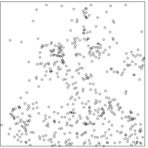
Figure 1.2: The Australian dataset (units in meters) –colour coded, to rep-resent each of the 67 species.

to regenerate after their shoots have been destroyed by fire [Illian et al., 2009]. These plants have extensive root systems from which the new shoots sprout, hence the term resprouters. The seeders are also specially equipped for regeneration from stress from fire. The fire stimulus causes these plants to shed their seeds which are able to germinate after the fire.

(22)

pockets of nutrients are located in the soil. Futhermore, the exudate from cluster roots chemically modify the surrounding soil climate [Lambers et al., 2012, Roelofs et al., 2001]. These compounds include organic anions, mu-cilages and water which facilitate the mobilization of nutrients from the soil. These physiological features will be referred to in Chapters 3 and 4 where the spatial locations of resprouter species are modelled. Spatial analyses will be conducted on three plant species in this dataset. Two of these species, are resprouters, whereas the third species is a seeder (familyEricaceae).

Most of the members of Ericaceae are associated with a mycorrhizal soil fungus [Sivasithamparam et al., 2004]. This association is formally classified as an ‘ericoid’ relationship. These types of symbiotic relationships, or ‘eri-coid mycorrhiza’, are vital for the survival of plants of the family Ericaceae especially in nutrient stressed environments. In particular, members of the familyEricaceae act as hosts providing carbohydrates and in turn obtain nu-trients from the network of fungal threads entwined around its roots [Watt and Evans, 1999]. This feature will be referred to in Chapter 3 where the spatial location of a reseeder is modelled.

(23)

pressures) can be compared. This would provide an insight into the effect of environmental heterogeneity on these species interactions. Furthermore, the estimates obtained in this analysis could serve as a biodiversity benchmark or standard reference for interactions within and between the species being studied.

Quantification of the interactions between and within the species groups would aid the understanding of the inherent relationships (in the associated ecological communities), and provide insight into the ecological importance of each species their contribution towards their coexistence.

1.2.2 Barro Colorado dataset

These data represent plants from a rainforest in Barro Collorado Island (BCI) in Panama, observed at 120m in altitude. The data were made available through the BCI forest dynamics research project [Hubbell et al., 2005] and are accompanied by soil maps providing information on the level of selected soil nutrients at specific quadrats within the survey site. The site, which has been established since 1980 is a 50 hectare plot and contains over 350,000 sampled trees [Condit, 1998, Hubbell et al., 1999, 2005] (see Figure 1.3). The plot is coordinated by the Centre for Tropical Forest Science of the Smithsonian Tropical Science Institute.

(24)

[image:24.595.248.392.125.240.2]

Figure 1.3: Barro Colorado Island (BCI) plot of 50 Hectares (demarcated by red square).

[Condit et al., 2010]. For this analysis we use the soil Phosphate level as the environmental covariate. The univariate point pattern representing this species consists of 2740 points, and represents a sampling area of 50 hectares of shape 1000m x 500m. Note that unlike the Australian dataset where the soil conditions were uniform, this dataset exhibits environmental heterogenity [Svenning et al., 2004].

1.3 Point process theory

Point process models facilitate the analysis of point patterns generated from the locations of objects in space. In particular, point processes offer the means to quantify short range interactions between the objects represented by these points and to also describe the geometry of the structure of the point pattern [Diggle, 1983, Bartlett, 1974].

(25)

[image:25.595.205.348.125.332.2]

Figure 1.4: Trunk of plant of Protium panamense with stilt roots (photo by R. Perez).

2008] from which spatial point patterns can be generated. For any given point process, different realisations of that process may lead to different point patterns. Despite the difference in the patterns, there would however be a similarity in their structure. The simplest point process is the homogenous Poisson process which is considered to be the reference/null model in point pattern analysis and is a building block for the construction of other point process models.

(26)

1.3.1 The homogeneous Poisson point process

The homogeneous Poisson process (HPP) generates point patterns which exhibit complete spatial randomness or CSR [Diggle, 1983] and is the ‘cor-nerstone’ on which point processes are built. A homogeneous Poisson point process, P, possesses a constant intensity, λo. The term λo represents the expected number of points per unit area in the pattern and has a Poisson distribution where the location of each point within the pattern is indepen-dent of the other points. This means that they do not exert any interaction on each other [Cressie and Wikle, 2011]. This point process is considered to be the null model in point process statistics. In particular, several point pattern diagnostic tests involve the comparison of a given point pattern V

to that generated from a homogeneous Poisson point pattern, P. This gives rise to information on the specific characteristics ofV in relation to P.

Formally, the Poisson process P on a point pattern Q, with intensity λo, has the following properties:

1. For B1, ..., Bn, disjoint bounded subsets of Q, {N(B1), ..., N(Bn)} are independent (where N(Bi) denotes the number of points inBi), and

2. For a bounded subset Bi, N(Bi) has a Poisson distribution with the intensity parameter λo = λi||Bi||, where ||.|| represents the Lebesgue measure andλi denotes the intensity of the subset Bi.

(27)

(a) (b)

Figure 1.5: Point patterns derived from (a) a homogeneous Poisson process, and (b) a bivariate homogeneous Poisson process. Note that each univariate point process is denoted by a separate symbol.

(28)

1.3.2 The inhomogeneous Poisson point process

The intensity for a homogeneous Poisson process has been described as being ‘uniform’ or ‘homogeneous’. In contrast, if the intensity for a point process is not uniform, the point process is characterised as an inhomogeneous point process [Baddeley, 2008]. This type of process is generated when inhomo-geneity (in the point intensity) is applied to a homogeneous Poisson point process. For a point pattern generated in this situation, the intensity of points is not constant throughout the point pattern like in the homogeneous case. For such a point pattern, the intensity is expressed as a function of location. Figure 1.6(a) depicts a point pattern derived from an inhomoge-neous Poisson point process. The corresponding density plot is shown in Figure 1.6(b). In this example, the intensity was expressed as a function of distance. The function used is:

f(x, y) = 100(√x+y)

(29)

(a) (b)

Figure 1.6: Illustration of (a) a point pattern derived from an inhomogeneous Poisson process, and (b) the density plot for the pattern in (a).

1.4 Point process data – point patterns

(30)

point pattern comprised of points which are not spatially distributed in a systemmatic fashion, that is, it exhibits neither clustering nor regularity. In addition, there is no dependence between the points such that each point occurs independently of the other points. This implies that there is no in-teraction between the objects which are represented by the points in the pattern.

(31)

1.4.1 Marked point patterns

For a given point pattern, each point represents one object/event. Additional information on each object (apart from its spatial location) may also be available. This additional information or ‘mark’ [Baddeley, 2008], associated with each point is considered to be an ‘attribute’ of that point. Baddeley [2008] notes that a mark can be thought of as an additional coordinate for each point in the spatial pattern.

A point pattern representing points which possess such additional in-formation is classified as a marked point pattern. Examples of such point attributes are: tree diameter breast height, number of eggs in nest, weight of eggs, animal/plant species and soil Phosphorus level. Note that marks can be qualitative/categorical such as species or quantitative/continuous such as tree height. If the marks are qualitative, the marked point pattern is a mul-titype point pattern. This point pattern would be associated with different subpatterns, each representing one particular mark of the mark type. An example of this is a point pattern representing different plant species such that the mark is a quantitative discrete mark corresponding to the species of the plant (as in Figure 1.5(b)). Mathematically, for a given marked mul-titype point pattern x in a bounded region in space W, with n individual marks, there existsn subpatterns, x1:n such that x={x1, ...xn}. Finally, a

(32)

1.4.2 Characteristics of point patterns

Point patterns may be described using first, second and higher order sum-mary statistics or characteristics. First order summary statistics are analo-gous to the concept of a mean in conventional statistics. In particular, first order characteristics relate to the spatial density of the points in a given point pattern. A homogeneous point pattern has a constant ‘intensity’ or density of points and an inhomogeneous point pattern a non-uniform intensity - in which case, the intensity is typically expressed as a function of location.

Second order summary statistics are analogous to the concept of disper-sion in conventional statistics since they relate to the proximity of the points to each other and hence their ‘interactions’. These summary characteristics provide valuable insights into the distribution of points at a specified range of distances and as a result the nature of the ‘interactions’ amongst points at these distances/ranges.

(33)

1.4.3 Point pattern first order summary

characteris-tics

The first order summary characteristic (statistic) for a point pattern describes the intensity of the points. If the pattern is a realisation of a homogeneous Poisson process, the first order characteristic is constant.

Let P denote a homogeneous Poisson process in a bounded window, W, with disjoint subsets Bi, i = 1, ..., n, such that P = Sn_i₌₁Bi. Notationally, for a point pattern x, realised fromP, the expected number of points forBi is proportional to the area ofBi where the constant of proportionality is the intensity denoted byλo. This can be expressed as

E[N(Bi)] = area(Bi)λo.

Note that the unbiased estimator of the true intensity λo is the empirical density of the points, ¯λo. This is expressed as

¯

λo =

n(x) area(W)

where n(x) represents the total number of points in the point pattern x.

(34)

λo(u) such that

E[N(Bi)] =

Z

Bi

λo(u)du ∀Bi ⊆W.

We now discuss some of the more commonly used second order summary statistics.

1.4.4 Point pattern second order summary statistics

The two most commonly used summary statistics relating to second order characteristics in spatial statistics are Ripley’s K function, K(r), and the pair correlation function, g(r) [Law et al., 2009, Baddeley, 2008, Mecke and Stoyan, 2005, Diggle, 1983]. The second order summary statistics are a means of providing summary information on the spatial distribution of points over a variety of scales [Stoyan and Penttinen, 2000]. Ripley’s K function and the pair correlation function, together with the cross pair correlation function, will form part of the exploratory analyses used in the analyses to follow.

1.4.4.1 Ripley’s K function

(35)

counted. This can be summarized as:

K(r) = λ−_o1E[#of points within distance r of a randomly chosen point].

The estimation of the K function for a given pattern at a specified distance

r, is achieved by calculating the mean number of points within a disc of radius r, from each point. Notationally the estimator of Ripley’s K function is expressed as:

ˆ

K(r) = N

−1P

i

P

j6=iI(dij < r) ˆ

λ (1.1)

where N denotes the number of points observed, dij the distance between points i and j, and I(ν) the indicator function which is equal to 1 if ν is true and 0 if ν is false. In addition, ˆλ =N/A, where A represents the area of the observation window. Note that the theoretical value of the K(r) for a homogeneous Poisson process is πr2_.

(36)

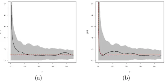
upper and lower limits of the envelope bands represent the minimum and maximum values of the K function estimated at each value of r, for the simulated patterns [Illian et al., 2008]. Clearly, the K curve for the observed data is consistently higher than that of the theoretical curve (including the simulation envelope), signifying clustering at all radiir≤0.25.

Figure 1.9 shows the estimated K function for the regular point pattern in Figure 1.7(b). The K curve for this pattern at the interaction radius/distance of 0.05m, is lower than that of the theoretical curve. In addition the curve lies outside the simulation envelope at this radius, indicating inhibition. We note however that above this distance (of 0.05m), the curve falls within the simulation envelope. This suggests that the pattern is random at distances above 0.05m. In summary the K function is valuable in that it provides a description of a given point pattern at various scales of distance, especially since many point patterns exhibit clustering at larger scales and regularity at smaller local scales [Dixon, 2002]. In addition Ambler and Silverman [2004] note that the clustering structure of some patterns may vary across scales. Examples of this include patterns with clusters of regularly spaced points or patterns with regularly spaced clustered points.

(37)

Figure 1.8: The K function for the clustered point pattern in Figure 1.7(c) with a simulation envelope representing 1000 simulations of a point pattern with CSR. The solid line denotes the estimated K function and the dotted line denotes the theoretical curve for a homogeneous Poisson process.

function λo(u) for any given pointu inx, this function is defined as

Ki(r) = n

X

xj∈x

λ−_o1(xj)E[#of points within distance r of xj]

for all points, xj:n in x. Note that the theoretical value of the Ki(r) for an inhomogeneous Poisson process is πr2. If the point pattern is spatially homogeneous, this function reduces to the K function for a point process with constant intensity.

1.4.4.2 Pair correlation function

(38)

Figure 1.9: The K function for the regular point pattern in Figure 1.7(b) with a simulation envelope representing 1000 simulations of a point pattern with CSR. The solid line denotes the estimated K function and the dotted line denotes the theoretical curve for a homogeneous Poisson process.

functiong(r) is defined as:

g(r) =K0(r)/2πr ∀r≥0,

whereK0(r) denotes the derivative of Ripley’s K functionK(r), with respect tor [Stoyan and Penttinen, 2000, Baddeley et al., 2007].

(39)

and the points in the pattern would vary – in other words, the (focal) plant’s eye view of the community varies. The pair correlation function summarizes this information for all the points in the pattern at a range of distances. For

Figure 1.10: A plant’s eye view of the community: the central focal point (solid disc at center of pattern) represents a focal plant within four discs of different radii (0.05m, 0.1m, 0.3m, and 0.6m). The radius of each disc represents the distance r for which the pair correlation function would be estimated. Each disc in turn represents that particular plant’s eye view of the community represented by the other points in the point pattern. For example, at the distance, 0.1m, there are six plants (points) in the community which are 0.1m from the focal point: this count varies for the different discs and hence the plant’s eye view varies with distance.

(40)

points within the specified distancer, indicating that this value ofris a hard core radius (see Section 1.5.2).

First, we consider a point pattern simulated from a homogeneous Poisson point process. This is the same pattern illustrated in Figure 1.7(a). The pair correlation plot for this pattern is shown in Figure 1.11, indicating that the values of the estimated pair correlation function fall predominantly on the Poisson reference line of 1. This reference line represents the plot of the pair correlation function of a point pattern exhibiting CSR. The plot of the estimated pair correlation indicates that the points are distributed independently from each other and the pattern exhibits complete spatial randomness.

We now consider the pair correlation functions for two point patterns, one regular, and the other clustered. These are the point patterns shown in Figures 1.7(b) and 1.7(c). The plot of the pair correlation function for the regular point pattern is shown in Figure 1.12. From this plot it is observed that the points for the pair correlation function fall predominantly below 1 for radii less than 0.05m. This attests to a pattern which reflects inhibition or regularity at distances r <0.05m.

(41)

Figure 1.11: Illustration of the pair correlation function for the pattern de-picted in Figure 1.7(a) with a simulation envelope representing 1000 simula-tions of a point pattern with CSR. The solid line denotes the estimated pair correlation function and the dotted line denotes the theoretical curve for a homogeneous Poisson process.

intensity, the inhomogeneous pair correlation function, gi(r), would be more appropriate than the pair correlation function discussed above. This function provides a summary of the dependence of points in a point pattern which does not contain a constant intensity and is related to the inhomogeneous K function. This function is expressed as:

gi(r) = Ki

0₍_r₎

(2πr)

(42)

Figure 1.12: Illustration of the pair correlation function for the pattern de-picted in Figure 1.7(b) with a simulation envelope representing 1000 simula-tions of a point pattern with CSR. The solid line denotes the estimated pair correlation function and the dotted line denotes the theoretical curve for a homogeneous Poisson process.

1.4.4.3 Cross pair correlation function

The cross pair correlation function describes the spatial dependence of points of different discrete marks/types at a range of distances, and provides an indication of the nature of the marks of neighbouring points for a typical point in a given multitype point pattern [Law et al., 2009, Illian et al., 2008]. Note that by convention, a marked point pattern with discrete marks is referred to as a multitype point pattern.

(43)

Figure 1.13: Illustration of the pair correlation function for the pattern de-picted in Figure 1.7(c) with a simulation envelope representing 1000 simula-tions of a point pattern with CSR. The solid line denotes the estimated pair correlation function and the dotted line denotes the theoretical curve for a homogeneous Poisson process.

cross pair correlation function is a smooth function of distance. We follow Law et al. [2009] and define this kernel as:

k(||$|| −r) =



  

  

(2h)−1_, _if _r₋_h_{≤ ||}_$_{|| ≤}_r₊_h

0, otherwise

(1.2)

where $ = xi −xj which represents the displacement between the points

xi, xj ∈ x and h represents a bandwidth parameter. We denote W$ as a translation of the window W such that

(44)

In addition, we denote A$ as the weight associated with the displacement

$ for the pair of pointsxi and xj such that A$ =W ∩W$. The cross pair correlation functionϑ(r), is then expressed as:

ϑ(r) =

6

=

X

xi,xj∈W

Iab(mi, mj)Φ 2πrA$

whereIab(mi, mj) represents the indicator function such that

Iab(mi, mj) =



  

  

1, if mi =a, mj =b

0, otherwise

and Φ represents the kernel function in Equation 1.2.

The cross pair correlation function is normalised using the intensities λa and λb which correspond to the intensities of the subpatterns xa and xb

respectively. The normalised form of the cross pair correlation functionχ(r) is expressed as:

χ(r) = 1

λaλb

ϑ(r).

When there is no spatial dependence between the marks, χ(r) ≈ 1, whereas values greater than or less than one indicate attraction and repulsion respectively. The cross pair correlation can take any nonnegative value. In addition, a value of 1 signifies ‘no spatial dependence’– as obtained from a point pattern simulated from a bivariate homogeneous Poisson process.

(45)

in the plot represents the empirical cross pair correlation function and the dotted line represents the cross pair correlation plot for a bivariate point pattern simulated from a homogeneous Poisson process. For the bivariate pattern in Figure 1.14(a), we note that there appears to be no interaction between the points of different marks. This is indicated by the fact that the plot lies predominantly on the Poisson reference line for this point pattern.

In contrast, Figure 1.15 shows a bivariate point pattern (and correspond-ing cross pair correlation plot) where the marks are discrete and there is de-pendence between the marks. The point pattern is shown in Figure 1.15(a) and the plot of the cross pair correlation function is shown in Figure 1.15(b). In this example, the marks appear to be dependent between 0.05 and 0.10 distance units and also at a distance of 0.13 units. This is evidenced by the fact that the solid line in Figure 1.15(b) lies above the Poisson reference line and simulation envelopes at this distance range. The empirical cross pair correlation function and the Poisson reference line (cross pair correlation plot for a bivariate point pattern simulated from a homogeneous Poisson process) are denoted by solid and dotted lines respectively.

1.4.4.4 Multitype K function

(46)

(a) (b)

Figure 1.14: Plots showing (a) a bivariate point pattern with discrete marks ‘A’ and ‘B’ (denoted by open circles and triangles respectively) in an ob-servation window of unit square area, and (b) the corresponding cross pair correlation plot (solid black line). The dotted line represents the cross pair correlation plot for a realisation of a homogeneous bivariate Poisson process. In addition, the cross pair correlation plot is accompanied by simulation en-velopes generated from 1000 realisations of a homogeneous bivariate Poisson process.

(47)

(a) (b)

Figure 1.15: Plots showing a bivariate point pattern and the corresponding cross pair correlation plot. The plot (a) depicts a bivariate point pattern with discrete marks ‘A’ and ‘B’ (denoted by open circles and triangles respectively) in an observation window of unit square area. Note that this point pattern is an example of a bivariate point pattern such that there is dependence between the marks. The plot (b) shows the corresponding cross pair correlation plot (solid black line). The dotted line represents the cross pair correlation plot for a realisation of a homogeneous bivariate Poisson process. In addition, the cross pair correlation plot is accompanied by simulation envelopes generated from 1000 realisations of a homogeneous bivariate Poisson process.

1.4.5 Cox processes

Cox processes model clustering or aggregation due to observed or unobserved environmental variables [Illian et al., 2010, 2008, Stoyan and Penttinen, 2000, Diggle, 1983]. Unlike Markov processes which are discussed in Section 1.5, Cox processes do not model local interactions.

(48)

Figure 1.16: Plot for the multitype K function for a bivariate point pat-tern generated from a bivariate homogeneous Poisson process (solid black line). The dotted line represents the plot of the multitype K function for a realisation of a homogeneous bivariate Poisson process. The accompanying simulation envelopes are generated from 1000 realisations of a homogeneous bivariate Poisson process.

commonly called a ‘random field’ or ‘random intensity function’ and can be plotted as a three dimensional surface.

(49)

1.5 Markov (Gibbs) point processes

For this thesis we focus on modelling not only the spatial positions of the organisms involved, but also the interactions (or dependence) between these organisms, thus necessitating point processes such as Markov point processes. Markov point processes model point patterns created in part due to under-lying interactions between the objects representing the points contained in the point pattern [Baddeley and Turner, 2000, Stoyan and Penttinen, 2000, Illian et al., 2008, Baddeley, 2008]. Comas and Mateu [2007] remark that these point processes are very suitable for modelling point patterns with a spatial structure that has been generated primarily from interpoint interac-tions. They note further that these models are useful in providing information on the empirical structure of forests, for example. In particular, interactions underlying these patterns can be quantified such that the relative strength of the interactions can be ascertained.

A Markov point process P, with density f(.) on datax, satisfies thelocal Markov condition such that forf(x)>0 and u /∈x, the ratio

λ(u|x) = f(x∪u)

f(x)

(50)

intensity [Baddeley and Turner, 2000, Kallenburg, 1984, Besag et al., 1982, Papangelou, 1976] of a point processP, for data x, can be described as the probability that there is a point u in P, bounded in region W, conditional on the fact that the process coincides with x (or given all the points in the point pattern are present).

Generally, point processes contain an intractable normalising constant which makes it difficult to evaluate the corresponding likelihood. It is usu-ally impossible to calculate the normalising constant analyticusu-ally even for the simplest of Markov processes. This is due to the fact that this involves eval-uating complicated multiple integrals [Baddeley and Turner, 2000, Baddeley and Lieshout, 1995]. For example, for a Markov process of densityf(x) with 2 intensity parameters (θ1, θ2) and 3 interaction parameters (θ3, θ4, θ5) such that, θ ={θ1, θ2, θ3, θ4, θ5}, the normalising constant is expressed as a func-tion ofθ as a five dimensional integral. An alternative to the likelihood is the pseudolikelihood which has as its building block the Papangelou conditional intensity.

(51)

1.5.1 Deriving the pseudolikelihood of a Markov point

process

Typically, for Markov processes, the pseudolikelihood is used for parameter estimation. This is, as discussed earlier, because the likelihood is analyt-ically intractable. The construction of the pseudolikelihood necessitates a Papangelou conditional intensity, which, for any univariate Markov process bounded in region of spaceW, with density function f for a pointu inWin standard form is expressed as:

λ(u;x) = f(x∪ {u})

f(x) (u /∈x)

λ(xi;x) =

f(x)

f(x\{xi})

(xi ∈x)

The pseudolikelihood contains the product of the conditional intensities of each point in x. In particular, Baddeley and Turner [2000] describe the pseudolikelihood as being an infinite product of infinitesimal conditional in-tensities. Mathematically the pseudolikelihood is expressed as:

P L(x,θ) = Y xi∈W

λ(xi;x)

!

exp

−

Z

W

λ(u;x)du

. (1.3)

(52)

[image:52.595.254.384.338.462.2]

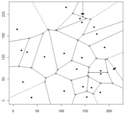
approximation. Baddeley and Turner [2000] describe the use of the Berman-Turner technique to approximate the integral in Equation (1.3) using a finite sum. The data is first augmented with ‘dummy’ points and a Dirichlet tes-selation (or Voronoi diagram) is obtained from the data and dummy points combined. A Dirichlet tesselation generates polygon regions in space each containing only one generating point (either a data or dummy point). As an example, Figure 1.17 illustrates a Dirichlet tesselation of points in point pattern representing Banksia menziesii from the Australian dataset. Each

Figure 1.17: Dirichlet tesselation of points represented by plants of Banksia menziesii

point (data and dummy) is associated with a quadrature weight. This is calculated as the area of the Dirichlet tile containing that point.

Using the quadrature weights, the integral is approximated such that:

Z

W

λθ(u;x)du≈

J

X

j=1

λθ(uj;x)wj

(53)

The log pseudolikelihood is therefore approximated as:

logP L(θ;x)≈

n(x)

X

i=1

logλθ(xi;x)− J

X

j=1

λθ(uj;x)wj.

Given that {uj, j = 1, ..., J}includes the data point {xi, i= 1, ..., n}, the log pseudolikelihood can then be rewritten as:

logP L(θ;x)≈

J

X

j=1

(yjlogλj−λj)wj (1.4)

where J represents the total number of points (data and dummy). Given

wj which denotes the weight per point j, yj is evaluated as _wj1 if the point under consideration is a data point and zero if it is a dummy point. This log-pseudolikelihood, logP L(θ;x), is formally equivalent to a log-likelihood of a weighted Poisson model where λj = λθ(uj;x) and yj and wj denote Poisson variables and quadrature weights respectively.

1.5.2 Pairwise interaction point processes

Pairwise point processes model only inhibitory interactions between objects represented by points on a given point pattern. The Strauss point process is the simplest of this class of processes and has a constant intensity and interaction. For a univariate point pattern, x, intensity parameter, β, and interaction parameter,γ, the likelihood for a univariate Strauss point process [Baddeley and Turner, 2000] is expressed as:

(54)

whereαis an intractable normalizing constant andsis a pairwise interaction function. This interaction function is expressed as:

s(x) = X i<j

h(||xi−xj||) (1.5)

such that

h(||xi−xj||) =I(||xi−xj||< r). (1.6)

The Euclidean distance between points xi and xj is denoted ||xi −xj|| and

I represents the indicator function. This interaction function (see Equation 1.5) computes the number of the ordered pairs of points which are within

r units of each other. The interaction parameter γ is such that γ ∈ [0,1]. Valuesγ that are between 0 and 1 signify a pattern with inhibition between points. If γ = 0, the point process is assumed to be a hard core process such that no two points in the respective pattern are within a distance of r

units apart. No interaction exists within a pattern for which γ = 1. In this situation the process is equivalent to a homogeneous Poisson process.

Recall that the conditional intensity for a Markov point process for a point u∈W is expressed as:

λ(u;x) = f(x∪ {u})

f(x) (u /∈x).

For the Strauss process, this is expressed as:

λ(u;x) = αβ

n(x)+1_γs(x∪{u})

(55)

which can be simplified as:

λ(u;x) =βγt(u;x)

where the function t(u;x) represents the number of points in x which are within a specified distance r from the point u. Mathematically t(u;x) is expressed as:

t(u;x) = #{xi ∈x:||xi−u|| ≤r}.

The conditional intensity for a Markov process for a point xi in x is expressed as:

λ(xi;x) =

f(x)

f(x\{xi})

(xi ∈x).

= αβ

n(x)_γs(x)

αβn(x)−1_γs(x\xi)

=βγt(xi;x).

Substituting the conditional intensities into Equation (1.3), the pseudolike-lihood,P L(β, γ;x), for the univariate Strauss process, which can be written as:

P L(β, γ;x) = n(x)

Y

i=1

βγt(xi,x)exp

−β

Z

W

γt(u,x)

=βn(x)γ2s(x)exp

−β

Z

W

γt(u,x)

.

(56)

1.5.3 Pairwise interaction point processes with a smooth

interaction function

The pseudolikelihood of a pairwise interaction point process, denotedJ, with a smooth interaction function has a similar structure to that of a Strauss point process. The only difference lies in the specification of the functions

s(x) and t(u;x). In particular, the function h in Equation (1.6) is replaced by a smooth function which is discussed later in more detail.

Recall that for the Strauss process, the function s(x), as described in Equation (1.5), obtains the sum of the ordered pairs of points in x which are withinr units of each other. Similarly, for this process t(u;x) represents the points in xwhich are within a specified distance r from a given point u

within a bounded windowW. For these functions, the interaction computed per pair of points (within r units apart) is a constant term, 1. If the points are not withinr units apart, the value attributed to that pair is 0, indicating that the interaction between the objects represented by these two points is of magnitude 0.

In stark contrast, for the point process J, the interaction computed per pair of points (whether or not they are within r units apart) is expressed as a function of the euclidean distance between the two points. This is achieved through the use of a smooth interaction function such as that proposed by Illian et al. [2009]. We follow this approach and expresss(x) for a univariate point pattern as:

s(x) =X i<j

(57)

where kxi−xjk represents the Euclidean distance d between the points xi and xj where i < j. We specify the function h of the form:

h(d) =



 

 

(1−(d/r)2₎2 _if ₀_{< d}_≤_r_; 0 otherwise,

for a fixed interaction radius r.

Similarly, we express t(u;x) for a univariate point pattern as:

t(u;x) = n

X

i=1

h(||xi −u||)

for points xi ∈x.

Note that the effect of the smooth interaction function is that the magni-tude of the computed interaction between plants is not constant (as for the traditional Strauss process), but decreases with increasing distance (Figure 1.18). Thus the interaction decreases smoothly with increasing distance from the given point.

1.5.4 Univariate area interaction point process

(58)

Figure 1.18: Plotted interaction functions showing change in interaction as distance between two specified points increase for an interaction radius of 25m.

the area of the union of discs associated with each point in the point pat-tern. Note that the radius of the discs is equal to the specified interaction radius of the process. The pairwise interaction processes are not suitable for modelling clustered patterns signifying attractive interactions. For modelling both attractive (positive) and inhibitory (negative) interactions we consider area interaction processes.

1.5.4.1 Probability density function

(59)

Lieshout, 1995] is defined in general form as

f(x)∝βn(x)γ−|Ux,r| _(1.8)

whereβandγare the intensity and interaction parameters respectively. Note that the interaction radius is denoted as r. The term |Ux,r|is expressed as

|Ux,r|= n

[

i=1

B(xi, r) (1.9)

where B(xi, r) is a disc of radius r centered at each data point xi [Baddeley and Lieshout, 1995] such that

B(xi, r) =

a∈ <2 :ka−xik ≤r .

Graphically, the term|Ux,r|is the area of the union of discs of radiusrcentred atxi [Baddeley and Lieshout, 1995, Baddeley and Turner, 2000, Picard et al., 2009].

The area of the union of discs is related to the interaction and is expressed as the decomposition of the union of grains,|Ux,r|, in an exclusion-inclusion style [Picard et al., 2009, van Lieshout, 2000]. It can be expressed as:

|Ux,r|= n(x)

X

i=1

|B(xi, r)|−

X

i<j

|B(xi, r)∩B(xj, r)|+...+(−1)n(x)+1

n(x)

\

i=1

B(xi, r)

. (1.10)

(60)

[image:60.595.223.414.180.361.2]

from a dataset which will be described later on in this Chapter.

Figure 1.19: The area of the union of discs of radius 2.5m, centered at points representing Banksia menziesii plants.

1.5.4.2 Conditional intensity

For the area interaction point process, the conditional intensity for a point

u∈Wand a point xi ∈xas:

λ(u;x) = f(x∪ {u})

f(x) =βγ

−B(u,r)\|U(x∪{u}),r| ₍_{u /}_∈_x₎ _(1.11)

and

λ(xi;x) =

f(x)

f(x\{xi})

=βγ−B(xi,r)\|U(x),r| ₍_x

i ∈x). (1.12)

(61)

[image:61.595.199.365.366.528.2]

condi-tional intensity (for u /∈x) is the additional area to the area of the union of discs contributed by a pointu. Figure 1.20 shows this area for a point u, de-noted by a filled circle, added to the point pattern in Figure 1.19. The points for the species Banksia menziesii are represented by open circles which are centered at the interaction discs corresponding to each point. The additional area incurred to the union area of the pattern (due to the addition of u) is shaded. We denote this area as the area of single occupancy, that is, the area of the disc which does not overlap with that associated with any other point.

Figure 1.20: Depiction of the additional area gained to the union of the area of discs centered at points representing Banksia menziesii.

1.5.4.3 Pseudolikelihood

(62)

an area interaction point process as:

P L(x,θ) = βn(x)γ−Pni=1B(xi,r)\|U(x),r|_exp

−β

Z

A

γ−B(u,r)\|U(x∪{u}),r|_du

,

(1.13) using the expressions for the conditional intensity for an area interaction pro-cess. For simplicity the pseudolikelihood for the univariate area interaction process is written as:

P L(x,θ) = βn(x)γ−ψ(x)exp

−β

Z

A

γ−ψ∗(u)du

(1.14)

whereψ(x) represents the sum of thesingle occupancy area of each point in the dataset and ψ∗(u) represents the additional area contributed by adding to the dataset the pointu /∈x. Note that the functions ψ(x) and ψ∗(u) are analogous to the functionss(x) and t(u,x) in the pairwise interaction point processes discussed earlier for pairwise interaction processes.

1.5.4.4 Area calculations

(63)

occupancy) between the disc associated with each point in a point pattern and the discs representing the remaining points. Figure 1.21 illustrates this further.

Other methods used to estimate the areas involved in analyses with area interaction point processes include the use of Voronoi tesselations together with a polygon clipping algorithm [Picard et al., 2009].

1.5.4.5 Interpretation and motivation

When γ = 1 the process reduces to a Poisson process. When 0< γ <1 the process generates an ordered pattern and when γ > 1 the generated point pattern is clustered. Baddeley and Lieshout [1995] identify area interaction point processes as being suitable for modelling specific biological processes. In particular, if the points represents animals or plants which utilize a food resource within a radius r, the organisms would tend to maximize the avail-able area of resource accessibility. As a result,|Ux,r|, the union of the area of the discs representing the points (or the total area of accessible food) would be maximized. This would lead to the interaction parameter, γ, being less than 1, signifying a relationship of inhibition between the organisms involved. In contrast, if the organisms are affected by a prey species, such that they are hunted within a radius r, these organisms would tend to minimize the area of their vulnerability to the prey, Ux,r, and hence the interaction parameter,

(64)

(a) (b)

[image:64.595.231.455.132.455.2]

(c)

(65)

1.5.4.6 Canonical form

We note that the canonical form of the area interaction point process is more easily interpretable than that of the standard form. This is due to the fact that in the standard form the intensity and the interaction parameters are positively correlated unlike the canonical case where they are negatively correlated. The correlation obtained in the canonical form then becomes analogous to that in the pairwise point processes where the correlation is also negative. As a result, we adopt the canonical form of the area inter-action point process as used in the R package, spatstat and van Lieshout [2006]. Note that in the canonical process the intensity parameterκ and the interaction parameter η are related to that of the standard form such that

β = κη and γ = ηπr12 _where _{β, γ} _{are the parameters used in the standard}

form of the area interaction point process.

Recall the conditional intensity for the standard form of the area inter-action point process in Equations (1.11) and (1.12). Substituting the trans-formed variables into these equations we express the conditional intensity of a pointu /∈x for the canonical form of the area interaction process as:

λ(u;x) = f(x∪ {u})

f(x) =κη 1−( 1

πr2)(B(u,r)\|U(x∪{u}),r|)

and for a pointxi ∈x we obtain:

λ(xi;x) =

f(x)

f(x\{xi})

(66)

For simplicity, we let

D(u) = 1

πr2(B(u, r)\|U(x∪{u}),r|)

and

D(xi) = 1

πr2(B(xi, r)\|U(x\{xi}),r|).

Note that D(u) denotes the normalised additional area (area of single oc-cupancy) incurred by the disc centered at a point u /∈ x to the area of the union of discs associated with the points in x. Similarly, D(xi) denotes the normalised additional area (area of single occupancy) incurred by the disc centered at a point xi ∈ x to the area of the union of discs associated with the points inx.

Note further that 1−D(xi) denotes the normalised area of multiple oc-cupancy (area of overlap) between the disc centered at the point xi and the union of the remaining discs associated with each point in the point pattern

x. Similarly, 1−D(u) denotes the normalised area of multiple occupancy (area of overlap) between the disc centered at the point u and the union of the discs associated with each point in the point pattern x.

We express the conditional intensity as:

λ(u;x) = f(x∪ {u})

f(x) =κη

(1−D(u)) _{u /}_∈_x _(1.15)

λ(u;x) = f(x∪ {u})

f(x) =κη

(1−D(xi)) _x

i ∈x. (1.16)

(67)

express the pseudolikelihood of the canonical form of the area interaction process as:

P L(x,θ) = κn(x)ηPni=1(1−D(xi))

exp

−κ

Z

A

η(1−D(u))du

. (1.17)

This is the canonical form of the expression in Equation (1.14).

Finally, we express Equation (1.17) substituting−C(xi) for 1−D(xi) and

−C(u) for 1−D(u) as further simplification to obtain:

P L(x,θ) = κn(x)ηPni=1−C(xi)

exp

−κ

Z

A

η−C(u)du

(1.18)

This can be further simplified as:

P L(x,θ) = κn(x)η−C(x)exp

−κ

Z

A

η−C(u)du

(1.19)

where Pn

(68)

1.6 Interaction radius specification

The estimation of the interaction radius has been described as being difficult and not straightforward [Møller and Waagepetersen, 2007, 2003, Baddeley, 2008]. The difficulty arises due to the fact that this model parameter is irregular and the resulting likelihood is not log concave as a function of the interaction radius [Møller and Waagepetersen, 2007, 2003]. Moreover, the statistical theory regarding the estimation of this parameter is unclear [Møller and Waagepetersen, 2007, Baddeley, 2008]. This is also reflected in the manual for the R package spatstat, used widely for point process model-ing. In the R documentation Baddeley [2008] states that interaction radius estimation cannot be done directly with the inherent point process functions in this R package. The interaction radius needs to be specified by the user.

The profile pseudolikelihood approach has been identified as one possible method for estimating the interaction radius [Illian et al., 2009, Baddeley, 2008, Møller and Waagepetersen, 2007, Bell and Grunwald, 2004, Møller and Waagepetersen, 2003]. The profile pseudolikelihood method is a modification of the maximum likelihood estimation method and facilitates the modeling of irregular parameters [Illian et al., 2009]. For a parameter vector θ =

{φ, R}, and data x, where R denotes the interaction radius parameter and

φ the regular parameters, the profile log pseudolikelihood (P LP(R,x)), is expressed as

P LP(R,x) = max

φ logP L((φ, R);x)

(69)

In particular, Baddeley [2008] adds that this method may or may not perform well.

To date, the most recently reported methods used for estimating the interaction radius when using Markov point processes are based on biological knowledge [King et al., 2012, Illian and Hendrichsen, 2010], visual inspection of exploratory plots such as the plot of Ripley’s K function [Picard et al., 2009] and the pair correlation function [Eckel et al., 2009], and the profile likelihood approach [Bell and Grunwald, 2004].

In this thesis we choose to specify the interaction radii based on biological background information to avoid confounding and complications related to the interaction radius estimation. Two datasets are considered. For the plant dataset, the interaction radii specified are based on biological background provided by Armstrong [1991] and cited by Illian et al. [2008]. Similarly, for the ant dataset, the specifications of the interaction radii are based on that used in previous analyses [Baddeley et al., 2006, Högmander and Särkkä, 1999].

1.7 Edge correction

If a point pattern, x, is considered to be the realisation of a finite process

P, defined only within the specified observation window,W, then the condi-tional intensity,λθ(u:x), ofP is observable within that window. If however,

(70)

realization ofP may fall on the edge of or outside of W. As a result of this, the conditional intensity of P may not be fully observed due to the pres-ence of ‘edge points’ and ‘unobserved’ data points outside of W leading to systematic error in parameter estimation.

Figure 1.22 illustrates the concept of ‘edge points’ and the effect of con-ducting an exploratory analysis (involving Ripley’s K function) in the pres-ence of ‘unobserved’ data. Figure 1.22(a) represents a simulated point pat-tern, A, subdivided into different zones. If, in reality, only the points denoted in red filled circles are observed, the resulting point pattern is B, depicted in Figure 1.22(c). Note that there are points in A (denoted in black filled circles) which are close neighbours of the points in red, but have not been ‘observed’, and are not included in B. This represents a situation where the data has been partially ‘observed’. The plots of the K function for A and B are shown in Figures 1.22(b) and 1.22(d). From visual inspection of these plots it is noted that there is a difference in the shape of the plots– however both plots suggest that the associated point patterns are clustered at inter point distances between 0 and 0.20 units.

The subpattern B, is reduced to a smaller point pattern, C, the points of which are denoted by red filled circles in Figure 1.22(e). This reduction is achieved by eliminating the points which are within 0.1 units from the border of B. This results in the exclusion of two clusters of points (‘edge points’) which are in B. For this example, we select the interaction radius of 0.10 units.

(71)

function for C and that for B is observed. Both plots however indicate that the associated point patterns are clustered. For C, the pattern appears to be clustered between distances of 0.02 and 0.13 units while that for B is clustered between distances of 0 and 0.20. In particular, the simulation envelope for the plot for C is larger indicating more uncertainty in the analysis. Overall, the differences observed indicate that the the presence of influential edge points (as with the two clusters of points in B which are excluded in C), and the size of the observation window chosen for data sampling may affect the plot of the K function (and other analyses) for the associated point patterns.

Two possible methods for edge correction are the border method or re-duced sample estimator [Illian et al., 2009, Baddeley and Turner, 2000, Hansen et al., 1999, Ripley, 1988] and reflection based methods [Baddeley and Turner, 2000]. For the point process P of finite interaction radius r, the border method applies the conditional intensity λθ(u :x) of P, to only

data points xi which are within r units from a random point u in W. The

pseudolikelihood is then formed over a ‘reduced sample’ or subregion of W, such that all the points in the subregion are within at leastr units from the boundary of W. This means that the pseudolikelihood is the product of the conditional intensities each evaluated at a corresponding retained point. The conditional intensity is not evaluated at the edge points–the edge points are used only as neighbours of the retained points. The reduced sample can be expressed as:

Wr ={u∈W :B(u, r)⊂W}

(72)

(a) (b) (c) (d)

(e) (f)

Figure 1.22: Illustration of (a) a point pattern subdivided into sampling regions with the points in one region denoted by red filled circles, (b) the plot of the K function for the point pattern in (a), (c) the point pattern formed by the points denoted by red filled circles in (a), (d) the plot of the K function for the point pattern in (c), (e) the point pattern in (c) subdivided into different regions with the points in one region denoted by orange filled circles, (f) the point pattern formed by the orange coloured points in (e), and the plot of the K function for the point pattern in (f). Each plot of the K function is accompanied by a simulation envelope derived from 1000 realisations of a homogeneous Poisson process. The solid black line represents the plot of the empirical K function and the Poisson reference line is denoted in red (dotted line).

(73)

[image:73.595.223.335.144.246.2]

Figure 1.23: Illustration of the reflection method using a point pattern (de-noted by black filled circles). The point pattern is reflected at the left and lower borders. In addition, one of the ‘surrogate’ point patterns (denoted by red filled circles) is also reflected at its left border.

neighbours for the ‘edge points’– however they also involve placing points in close proximity to each other without any background on the pattern structure [Illian et al., 2009, Pommerening and Stoyan, 2006].

Bayesian point process modelling of ecological communities

COMMUNITIES

Glenna Evans Nightingale

communities

Abstract

Declarations

Acknowledgements

Contents

Chapter 1

Background

1.1

Modelling ecological communities

1.1.1

Biodiversity – species coexistence and

interac-tions

1.1.2

Biodiversity – spatial dimension

1.2

Datasets

1.2.1

Australian dataset

1.2.2

Barro Colorado dataset

1.3

Point process theory

1.3.1

The homogeneous Poisson point process

1.3.2

The inhomogeneous Poisson point process

1.4

Point process data – point patterns

1.4.1

Marked point patterns

1.4.2

Characteristics of point patterns

1.4.3

Point pattern first order summary

characteris-tics

1.4.4

Point pattern second order summary statistics

1.4.5

Cox processes

1.5

Markov (Gibbs) point processes

1.5.1

Deriving the pseudolikelihood of a Markov point

process

1.5.2

Pairwise interaction point processes

1.5.3

Pairwise interaction point processes with a smooth

interaction function

1.5.4

Univariate area interaction point process

1.6

Interaction radius specification

1.7

Edge correction