components: asymptotic analysis and finite size
effects
Louise Reeve and Jonathan A.D. Wattis
School of Mathematical Sciences, University of Nottingham, University Park, Nottingham NG7 2RD, UK
E-mail: [email protected], [email protected]
Abstract. We consider the model of random sequential adsorption (RSA) in which two lengths of rod-like polymer compete for binding on a long straight rigid one-dimensional substrate. We take all lengths to be discrete, assume that binding is irreversible, and short or long polymers are chosen at random with some probability. We consider both the cases where the polymers have similar lengths and when the lengths are vastly different. We use a combination of numerical simulations, computation and asymptotic analysis to study the adsorption process, specifically, analysing how competition between the two polymer lengths affects the final coverage, and how the coverage depends on the relative sizes of the two species and their relative binding rates. We find that the final coverage is always higher than in the one-species RSA, and that the highest coverage is achieved when the rate of binding of the longer polymer is higher. We find that for many binding rates and relative lengths of binding species, the coverage due to the shorter species decreases with increasing substrate length, although there is a small region of parameter space in which all coverages increase with substrate length.
Keywords: Random sequential adsorption, asymptotic analysis, recurrence relations.
PACS: 68.43.Mn Kinetics of adsorption, 64.60.-i general studies of phase transitions, 64.60.an finite size systems
Submitted to: J. Phys. A: Math. Gen.
1. Introduction
effects which complicate such processes, with particular reference to applications in colloidal systems.
[image:2.595.149.521.293.388.2]An important technique in gene therapy is to deliver DNA into an defective cell’s nucleus, which can then go on to create a functional protein to treat a disease. DNA has many features which cause it to be spatially extended, one being the electrostatic repulsion between phosphates on its backbone. For DNA to be condensed, these negative charges must be neutralised. The original application motivating this present work is that of different lengths of positively charged polymers attaching to a negatively charged DNA to neutralise its charge, allowing it to condense and be transported into the cell’s nucleus. In experimental work, it has been found that DNA condenses when it reaches 90% neutralisation [12]. Since it is possible to design polymers with specific properties, our motivation is to design polymer mixtures to maximise coverage.
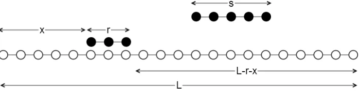
Figure 1. Diagram of polymer of lengthrbound to the substrate of lengthL, and a polymer of lengthsattempting to bind in the remaining gap of length L−r−x
RSA is also known as the ”Parking Problem” due to the similarity with trying to park a car on a street. This can be modelled in two ways: discrete or continuous substrates, here we focus on the discrete case. Our aim in this paper is to analyse random sequential adsorption (RSA) processes in which two distinct lengths of ‘polymer’ (r, s) which are assumed to be straight and rigid bind to a long straight rigid one-dimensional substrate, of lengthL(withL≫r, s) as summarised in figure 1. We are concerned with how the coverage (θ, with 0≤θ ≤1) depends on the length of the polymers concerned, and in particular, finite size effects.
In discrete RSA, the substrate has a discrete number of unit binding sites to which a polymer can bind. Where one polymer lands affects where others can land, as we assume that they cannot be removed once bound, and cannot overlap. Our main interest is the total coverage achieved by the polymers, that is, the proportion of the substrate occupied by polymers. Cornette et al.[6] show that total coverage approaches jamming exponentially in time. However, the jamming limit is not straightforward, as Bonnier
et al [3] analyse the pair correlation function for the adsorbed sites, revealing complex structure in the jammed state.
of generalised RSA systems have been covered: Tarjus et al. [26] have considered the effect of adding desorption and diffusion of adsorbed species on the substrate to RSA. They consider hard spheres being adsorbed onto a flat 2D surface. They use distribution functions to describe the kinetics of the process which, instead of the jamming limit, now approaches a dynamic equilibrium in which desorption rates balance adsorption. Maltsev et al. [19] consider reversible adsorption and motion on the substrate, in the case of a discrete one-dimensional substrate. In this simpler system, it is possible to analyse how the distribution of gaps between adsorbed polymers changes over time, and so describe the kinetics of adsorption. The addition of small rate of desorption allows higher coverages to be attained than in pure RSA.
Complexity above one-dimensional, but below two-dimensional have been considered by Baram and Kutasov [2], who consider a 2×∞ lattice. By using a master equation approach, they show that the jamming density is 1
2(1− 1 2e−
1
) = 0.408, significantly less than the one-dimensional case, which for dimers landing on a 1D discrete substrate gives φd = 1−e−2 = 0.86466, or for unit particles adsorbing onto
a continuous substrate gives R´enyi’s constant, φc = 0.7476. Feder’s approximation for
dimers on a two-dimensional substrate gives φ2
c = 0.5589 or φ
2
d= 74765 in the cases of
continuous and discrete substrate respectively.
Various aspects of the case where the binding species includes a mixture of lengths have been considered by Hassan and Kurths [13], Hassan et al [14], Burridge and Mao [4], and Purves et al. [22]. Hassan and Kurths [13], study the two-component RSA system with a continuous substrate. This is simplified by making one of the two binding species have zero length. They seek solutions for the pdes describing the gap
distribution in terms of a self-similar solution, obtaining the distribution of the form
t2 e−xt
. A similar system is studied by Hassan et al [14], where now both species have finite length, σ and mσ with 1 < m ≤ 2. After deriving the pdes for the evolution of
the gap length distribution, they present numerical results showing the total coverage against the probability of the shorter polymer binding. This is paper is the closest in spirit to the work we present below in Sections 2 and 3. Burridge and Mao [4] consider RSA in which the lengths of adsorbing species are drawn randomly from a distribution, again with the restriction that the longest possible polymer has to be less than twice the length of the shortest. They find exact analytic formulae for the coverage, whilst these expressions are confirmed against numerical simulations, they are too complicated to evaluate analytically.
Purves et al. [22] consider the scaling of coverage with availability of binding sites (A) in the jamming limit. They consider the case of two distinct lengths of binding species, hence there are two availabilities, Ar(t) for the shorter species and As(t) for
the longer. In the case of a discrete substrate, Ar(t) ∝ θ(∞)− θ(t), and As(t) ∝
[θ(∞)−θ(t)]n
where n depends on the relative rate of binding of the two species and the difference in their lengths. For the continuous substrate,Ar(t)∝[θ(∞)−θ(t)]2 and As(t)∝[θ(∞)−θ(t)]2exp−κ/[θ(∞)−θ(t)]. These scaling laws carry over to the
substrate give A ∝ θ(∞)−θ(t) for the discrete substrate and A ∝ [θ(∞)−θ(t)]2 for the continuous.
Feder [10] simulated the sequential filling of a surface by disks, and obtained the limit of 0.55 which is close to the square of R´enyi’s constant. Hinrichsen et al. [15] perform simulations of disks and line segments onto a two-dimensional substrate, obtaining the hole size distribution and coverage in the jamming limit. Viot et al. [28] consider the jamming limit for the case of various shapes of 2D objects being adsorbed onto a 2D surface. The coverage approaches its limit in algebraic fashion, namely
θ(∞)−θ(t)∼t−n
, with an exponent (n) that depends on the shape of the object being adsorbed. Whilst circular, and most other shaped objects show a standard asymptotic behaviour with n = 1/3, they find that for highly elongated shapes, they find the exponent n = 1/2, together with cross-over behaviour between this exponent and the standard asymptotic behaviour. Talbot and Schaaf [25] consider the adsorption onto a continuous two-dimensional substrate of a two-component mixture of circular disks with vastly differing sizes. By considering exclusion circles around each adsorbed disc, they deriving odes for the coverage due to each size of disc. These yield the approximate
behaviour of the system in the jamming limit, and in the case of the small discs becoming vanishingly small, the results are highly accurate.
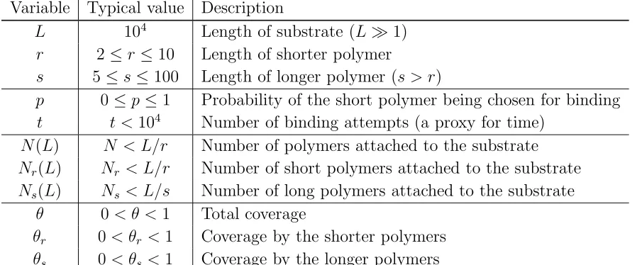
Variable Typical value Description
L 104
Length of substrate (L≫1)
r 2≤r ≤10 Length of shorter polymer
s 5≤s≤100 Length of longer polymer (s > r)
p 0≤p≤1 Probability of the short polymer being chosen for binding
t t <104
Number of binding attempts (a proxy for time)
N(L) N < L/r Number of polymers attached to the substrate
Nr(L) Nr < L/r Number of short polymers attached to the substrate Ns(L) Ns < L/s Number of long polymers attached to the substrate
θ 0< θ <1 Total coverage
[image:4.595.71.520.390.577.2]θr 0< θr <1 Coverage by the shorter polymers θs 0< θs <1 Coverage by the longer polymers
Table 1. Summary of parameters, variables and notation used in this paper.
shorter than the substrate. Conclusions are drawn and discussed in section 5.
1.1. One polymer case
The one-polymer formulation of RSA was first proposed by R´enyi [24]; in this model, the substrate is continuous and the expected density of cars parked on a street of infinite length is 74.75979%. For the case of a discrete substrate, the coverage depends on the length of binding species. Here we summarise the averaged results for the case of a single species of length r binding to a discrete substrate of length L.
To form the recurrence relation, we first observe that when the substrate length,
L, is less than that of the polymer, r, no polymers can bind. When L is between r
and 2r, only one polymer is able to bind. Once the length of the substrate reaches and exceeds 2r, the number of polymers bound, Nr, depends on the location that each prior
polymer has landed on the substrate. This is because the gap each side of the polymer could have size greater than or less than r. The equations governing jamming coverage are thus
N(L) = 0, (L < r), (1)
N(L) = 1, (r≤L <2r), (2)
N(L) = 1 + 2 (L−r+ 1)
L−r X
n=r
N(n), (L≥2r). (3)
Rearranging the latter equation yields
(L−r+ 1) [N(L)−1] = 2
L−r X
n=r
N(n). (4)
Now we apply the transformation L → L+ 1 and take the difference of the resulting equation and (4) to obtain the recurrence relation
(L−r+ 2)N(L+ 1) = (L−r+ 1)N(L) + 2N(L−r+ 1) + 1. (5)
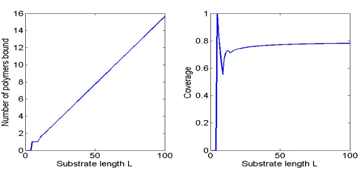
The coverage, θ, is defined to be the proportion of substrate sites that have polymer bound, and is calculated by θ(t) =rN(L)/L.
The first graph in figure 2 shows that once the substrate length passes a certain length, the relationship formed between the number of polymers bound and the substrate length is approximately linear. The second graph shows that, again after the substrate reaches a certain length, the coverages asymptote to just below 80% coverage. This value corresponds to the gradient of the curve in the first panel.
2. Two polymer case
In the case where polymers of two distinct lengths can bind to the substrate, we require two variables, Nr and Ns to describe the RSA process. We are interested in how the
Figure 2. Graphs obtained using the recurrence relation (5) for the one polymer case whenr=5. Left, the number of polymers bound to the substrate as the length of the substrate varies. Right, the coverage by the polymers as substrate length varies.
polymers. We denote the two lengths of polymer byrands, and usepfor the probability of the shorter polymer (r) binding, so that the probability of the longer polymer (s > r) binding is 1− p. Clearly, a stochastic process will give different coverages on each realisation; however, averaging over a large number of simulations leads to well-defined values for the coverage due to each species. We consider the kinetics of the binding process, using a time unit corresponding to the number of binding attempts. Using an alternative notation, we could define binding rates Kr for the r-polymers and Ks for
the s-polymers, then p=Kr/(Kr+Ks).
To understand the expected coverage of the stochastic process, we assume there is no cooperativity between the binding of short and short, or short and long, or long and long polymers, that is, each binding event is independent of the arrangement of polymers already bound to the substrate. We also assume that there is no specific spatial arrangement of bound polymers, so that it is sufficient to keep track of the total numbers of each type of polymer on the substrate, that is, a spatially averaged description of the substrate will suffice. These assumptions are similar to those made in the construction of ‘mean field’ models; hence the system of equations that we derive can be considered as mean field model of RSA. Whilst both Nr, Ns are functions ofL, r, s and p, we consider r, s, and p as fixed parameters, and focus on describing how
Nr, Ns depend on the substrate length variable, L. Firstly, we formulate equations for
each of Nr(L), Ns(L) when just the r-polymer binds
Nr(L) = 1 +
2 (L−r+ 1)
L−r X
n=0
Nr(n), Ns(L) = 0 +
2 (L−r+ 1)
L−r X
n=0
Ns(n), (L≥r).
relations
Nr(L) = 0 +
2 (L−s+ 1)
L−s X
n=0
Nr(n), Ns(L) = 1 +
2 (L−s+ 1))
L−s X
n=0
Ns(n), (L≥s).
(7) As well as the clear change in placement of the zero and one terms on therhss, equations
(6) and (7) differ in the denominator and the limits on the sums.
Multiplying (6) and (7) by p(L−r+ 1) and (1−p)(L−s+ 1), respectively, and adding, we obtain equations for the full process in which polymers are chosen at random to bind, namely
ΛNr(L) = p(L−r+ 1) + 2p L−r X
n=0
Nr(n) + 2(1−p) L−s X
n=0
Nr(n), (8)
ΛNs(L) = (1−p)(L−s+ 1) + 2p L−r X
n=0
Ns(n) + 2(1−p) L−s X
n=0
Ns(n), (9)
for L≥s, and where Λ = (L+ 1−s−ps+pr),
whilst for r≤L < s, we have (6a), and forL < r,Nr(L) = 0 =Ns(L). Since r < s, the
sums in (8) can be rewritten as
2p L−r X
n=0
Nr(n) + 2(1−p) L−s X
n=0
Nr(n) = 2 L−s X
n=0
Nr(n) + 2p L−r X
n=L−s+1
Nr(n). (10)
Since, in practice, L≫r, s, this means that the two sums over large numbers of terms are replaced by one sum over a large number of elements (0≤n≤L−s), and a second
sum, which includes a much smaller number of terms (L−s+ 1 ≤n≤L−r).
We transform (8) by making the substitutionL7→L+ 1 and take the difference of
the transformed equation and the original, together with the identity (10), to obtain
2Nr(L−s+ 1)−Nr(L+ 1) +p
= [L+ 1−s−pr+ps][Nr(L+ 1)−Nr(L)]
+ 2p[Nr(L−s+ 1)−Nr(L−r+ 1)], (11)
A similar method forNs(L) is used on (9), yielding
2Ns(L−s+ 1)−Ns(L+ 1) + (1−p)
= [L+ 1−s−pr+ps][Ns(L+ 1)−Ns(L)]
+ 2p[Ns(L−s+ 1)−Ns(L−r+ 1)]. (12)
The equations (11)–(12), are formally uncoupled, however, solutions to both are required for a full understanding of this two-component RSA system. Whilst (11)–(12) holds for
L ≥ s, for r ≤ L < s, we have just (6a) together with Ns(L) = 0, and for L < r, Nr(L) = 0 =Ns(L).
Given a solution for Nr(L), Ns(L), we calculate the coverages as
θr =
rNr(L)
L , θs=
sNs(L)
As L increases from zero, clearly the first polymer allowed to bind is an r-polymer, which can only bind once L ≥ r. Once L is of greater length than r, there are two cases which need to be considered. The first is (a) the possible binding of ans-polymer, which first occurs when L=s; the second, (b), occurs whenL= 2r, at which point it is possible for twor-polymers to bind, provided the first binds at one end of the substrate. In the special case s = 2r, both possibilities arise simultaneously at L = s = 2r. If
s < 2r then, as L increases, case (a) occurs before (b), that is, s-binding occurs first; whereas if s > 2r, then case (b) occurs before (a), and multiple r-polymers can bind before a single s-polymer. Both scenarios will be considered in the following sections.
3. Numerical simulations
3.1. Monte Carlo Simulations
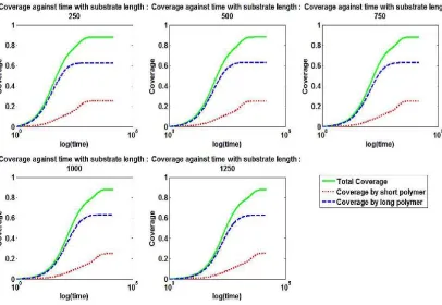
Monte Carlo simulations are extremely useful for modelling situations such as RSA. At each step in the simulation we choose either a long or short polymer, according the probabilityp, and attempt to land it on the substrate. If it finds a location of sufficient size, it binds to the substrate, making either r or s consecutive sites unavailable for binding. Once there are no stretches of free sites of length r or greater, then the simulation stops, no more binding events are possible, and the substrate is jammed. A count of the number of binding events is used as an effective time. The simulation is carried out many times, and an average coverage is calculated, with larger numbers of simulations leading to increased accuracy.
All five graphs in figure 3 show the coverage increasing as successive binding events are attempted. The results show similarly shaped curves, converging to the same limit, though when the substrate length, L, increases, the system takes longer to reach the final jammed state. In the case illustrated, p= 0.2, meaning that the shorter polymer has a lower probability of binding, and we note that the coverage by the shorter polymer takes a longer time to reach steady-state than the longer polymer. This is due to the short polymer filling in the gaps left by the longer polymer in the final stages of the transition to the jammed state.
We have performed simulations for a range of values for p, r, and s, recording the final coverage due to each polymer type. Graphs of coverage against p agree with the results plotted in figure 5, which is discussed in section 3.2. Figure 6 shows the coverages θ∗ plotted against substrate length, L, for the Monte Carlo simulations, and
two theoretical techniques: a full solution of the recurrence relation, and an asymptotic approximation outlined later.
3.2. Numerical solution of deterministic recurrence relation
Figure 3. Graphs obtained using Monte Carlo simulations for different lengths of the substrate, showing how the coverage by the polymers changes as RSA proceeds. Parameter values: r= 3,s= 5,p= 0.2, averages are taken over 1000 iterations.
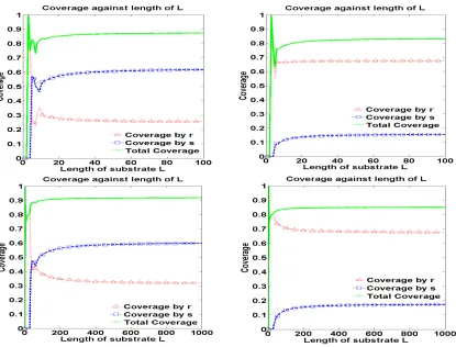
against substrate length for a range of polymer length ratios and relative binding rates, corresponding to the right panel of figure 2. In the upper panels of figure 4, r = 3 and
s= 5, so thatr < s ≤2r; whereas in the lower panelsr = 3 ands= 30, so thats >2r. On the left we have p = 0.2 so the longer polymer binds at a higher rate, and on the right, p= 0.8 so that the shorter polymer binds more rapidly.
In all cases the coverage due to the longer polymer, θs increase with substrate
length, L, as in the one-polymer case. However, in most cases, the coverage due to the shorter polymer, θr, decreases with increasing substrate length the dependence is not
clear in the case s = 5,p = 0.8 (the top right panel). The total coverage, θ = θr+θs
increases with substrate length in all cases. In the case of r= 3, s= 5 and p= 0.2, the total coverage is θ= 0.873, whenr = 3, s= 5 and p= 0.8, we have θ = 0.831, thus the total coverage is higher when the probability of choosing the shorter polymer is lower.
Higher total coverages are also found when the ratio of long to short polymer lengths is increased, whenr= 3,s= 30 andp= 0.2, the total coverage reachesθ= 0.918. These higher coverages are achieved when p, the probability of the smaller polymer binding, is small, which leads to an initial period of more rapid deposition of longer polymers. On a slower timescale, there follows a slower stage in which the smaller polymers fill in the gaps between the larger polymers.
Figure 4. Expected coverages θr, θs, θ (13) calculated from the recurrence relations (11)–(12) plotted as functions of substrate length,L. Upper panels: the case of similar lengths of binding species, r < s < 2r; lower panels: the case of vastly differing lengths,s >2r; left panels: the case of long species binding more rapidly than short; right panels: the case of short species binding more rapidly than long. Parameter values: top left: r= 3, s = 5, p= 0.2; top right: r = 3,s = 5, p= 0.8; lower left:
r= 3,s= 30,p= 0.2; lower right: r= 3,s= 30,p= 0.8.
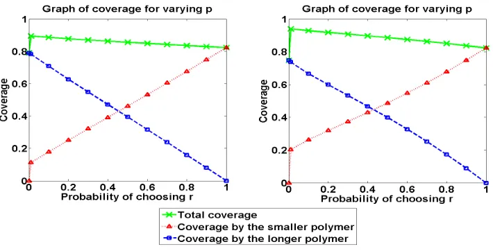
against probability of choosing the shorter polymer, p. On the left we show the results for the case of similar lengths 1 < s/r < 2, and on the right, the case of vastly differing lengths, that is, s/r > 2. The two graphs are qualitatively similar, and show an approximately linear dependence on p. There is a discontinuity at p = 0: when
p = 0, we have a one-polymer system, thus the maximum coverage will be about 75-80%. However, for 0 < p ≪ 1, there are two polymers, and the longer one binds on a quicker timescale, and the shorter one on the slower timescale, filling in the gaps left by the longer polymer, thus leading to significantly higher coverages.
4. Asymptotic Methods
The final method we use to calculate the solution of the recurrence relations (11)–(12) is asymptotic approximations. We consider two cases for the relative magnitudes of r
Figure 5. Graphs showing how the coverages of each polymer type changes withp, the probability of choosingr. Left, similar polymer lengths,r= 3,s= 5, andL= 1000; right, vastly dissimilar polymer lengths,r= 3,s= 30 andL= 1000.
with 1/r ∼ r/s ∼ s/L ≪ 1; and (ii) similar lengths, that is, r ∼ s. Case (ii) follows the theory outlined in [18] for the single component RSA; however, the addition of a second binding species significantly complicates the problem. In Case (i), we also follow the asymptotic approach of [18], but new scalings are required to account for the significantly different lengths of the binding species.
4.1. Polymers of dissimilar length
Clearly if r ≪s then the scaling r ∼s fails, so we require different asymptotic scaling from those used in [18]. Here, we consider the case where r ∼ s/r ∼ L/s ≫ 1. So we replace the variables in the recurrence relation (11) with the variables
r = 1
ǫ, s = b s
ǫ2, L=
y
ǫ3, Nr(L) = 1
ǫ2nr(y), Ns(L) = 1
ǫns(y), (14)
where bs, y, nr(y) and ns(y) are all O(1), with ǫ ≪ 1. This is due to our expectation
that, for 0 < p < 1, an O(1) amount of coverage will be due to each of the r- and
s-polymers, thus rNr = O(L) and sNs = O(L). We use primes to denote derivatives
(12), to obtain 2
ǫ2nr(y−ǫbs+ǫ 3
)− 1
ǫ2nr(y+ǫ 3
) +p
=
y
ǫ3 + 1−
b s ǫ2 −
p ǫ +
pbs ǫ2
1
ǫ2[nr(y+ǫ 3
)−nr(y)]
+ 2p
ǫ2[nr(y−ǫbs+ǫ 3
)−nr(y−ǫ
2 +ǫ3
)], (15)
2
ǫns(y−ǫbs+ǫ
3 )− 1
ǫns(y+ǫ
3
) + (1−p)
=
y
ǫ3 + 1−
b s ǫ2 −
p ǫ +
pbs ǫ2
1
ǫ[ns(y+ǫ
3
)−ns(y)]
+ 2p
ǫ [ns(y−ǫbs+ǫ
3
)−ns(y−ǫ
2 +ǫ3
)]. (16)
Next, we Taylor expand these equations using ǫ ≪ 1 which, after much cancellation, leads to
yn′
r(y)−nr(y) =−ǫbs(1−p)n′r(y) +ǫ
2
b s2
(1−p)n′′
r(y) +p+p n′r(y)
+O(ǫ3
). (17)
We note that (17) is inhomogeneous atO(ǫ2
) but homogeneous at O(ǫ).
Substituting nr(y) = Ar(s, pb )y+ǫBr(y,bs, p) into (17) means that (17) is satisfied
up to O(ǫ) for any value of the arbitrary ‘constant’ Ar. Expanding and rearranging
at next order in ǫ gives yB′
r(y)−Br(y) = −(1−p)bsAr, which can be solved using the
integrating factor 1/y2
to giveBr =−(p−1)bsAr, and hencenr(y) =Ary−ǫ(p−1)bsAr.
Substituting in the initial variables (14) into this solution, we obtain
Nr(L) = ArL
r
1 + s(1−p)
L
, (18)
where Ar =Ar(s/r2, p). Hence the coverage due to the shorter polymers is given by
θr(L;s/r, p) =Ar
1 + s(1−p)
L
, (19)
which decreases with increasing Lfor all values of p.
For the long polymers, Taylor-expanding (16) and simplifying gives
yn′
s(y)−ns(y) =ǫ(1−p)[1−bsn′s(y)] +ǫ
2
[(1−p)bs2−
pn′
s(y)] +O(ǫ
3
). (20)
The different scalings of r and s, Nr and Ns in (14) results in this differential
equation for ns(y) is quite different to that for nr(y), namely (17). Substituting ns(y) = Aes(bs, p)y+ǫBs(y;bs, p) into (20) leads to yBs′ −Bs = (1−p)(1−bsAes), which
yields the solution ns(y) =Aesy[1−ǫ(1−p)s/yb ]−ǫ(1−p). Substituting in the original
variables using (14) and Aes =r2As/s, we obtain
Ns(L) = AsL
s
1 + (1−p)s
L
Comparing (18) with (21), we note that there is an extra term at the end of (21) due to (20) being inhomogeneous at O(ǫ). The coverage due to the longer polymers is thus given by
θs(L;s/r, p) =As−
(1−As)s(1−p)
L , (22)
which increases with substrate length, that is, asL→ ∞; this result is in contrast with that for θr (19). Combining (19) and (22), we obtain
θ(L;s/r, p) =A−s(1−p)(2A−1)
L . (23)
[image:13.595.83.498.292.651.2]Hence the total coverage will always increase with substrate length, L, since the R´enyi constant for the mixed system, A=Ar+As, must satisfy A >1/2.
4.2. Assignment of constants, Ar, As
In the asymptotic solutions (18) and (21), (and later in equations (30), (31)), the arbitrary constants, Ar(s/r, p), As(s/r, p)), are leading order approximations to the
coverages θr, θs. From the graphs in figure 5, we note that the coverages are
approximately linear inp, and by comparing the two graphs, fors/r = 5/3 ands/r= 10, we note that the dependence on s/r is reasonably small.
We defineφr to be R´enyi constant for the discrete one-dimensional, one component
system with polymer length r in the limit L → ∞. As a function of p, the coverage
θs thus takes the value θs = φs at p = 0 and θs = 0 at p = 1; hence θs = (1−p)φs.
At p = 1, θr = φr; however, in the limit p → 0+ we have θr = (1−φs)φr, since in
this limit, the polymer will fill with s-polymers, leaving (1−φs) of the substrate free.
Then a proportion φr of this will be filled with r-polymers. Hence we approximate θr
by θr =pφr+ (1−p)(1−φs)φr, and simplifying,
Ar = (1−φs+pφs)φr, As= (1−p)φs. (24)
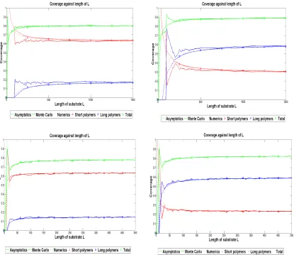
In figure 6 we compare all three of the methods used in this paper, namely, Monte Carlo simulations, a full numerical solution of the recurrence relations (11)–(12), and asymptotic solutions of these recurrence relations. The upper panels correspond to
r = 10, s = 100, with p = 0.2 and p = 0.8. Clearly in both graphs, the results differ at small L due to the asymptotic approximations being made on the assumption of
L ∼ r3 ≫
1. The asymptotic solutions and the numerical solution of the recurrence relations are difficult to distinguish on the two graphs. At larger values of L, all three solutions agree well. It is worth noting that in both graphs the coverage due to the longer species, θs, and the total coverage both increase with L; whilst the coverage due
to the shorter species, θr decreases withL. This is due to the fact that end effects cause
a slight increase in the likelihood of shorter polymers binding.
4.3. Polymers of similar length
For this approximation, where r and s are similar in magnitude, and where L ≫r we introduce a small parameter ǫ≪1 defined byǫ= 1/r. Then we rescale the variables in the recurrence relation with new variables bs, y, nr, and ns, all of which are O(1) and
are defined by
r= 1
ǫ, s= b s
ǫ, L= y
ǫ2, Nr(L) = 1
ǫnr(y), Ns(L) =
1
Using these definitions, the governing equations (11) and (12) become 2
ǫnr(y−ǫbs+ǫ
2 )− 1
ǫnr(y+ǫ
2 ) +p
=
y
ǫ2 + 1−
b s ǫ −
p ǫ +
pbs ǫ
1
ǫ[nr(y+ǫ
2
)−nr(y)]
+ 2p
ǫ [nr(y−ǫbs+ǫ
2
)−nr(y−ǫ+ǫ
2
)], (26)
2
ǫns(y−ǫbs+ǫ
2 )− 1
ǫns(y+ǫ
2
) + (1−p)
=
y
ǫ2 + 1−
b s ǫ −
p ǫ +
pbs ǫ
1
ǫ[ns(y+ǫ
2
)−ns(y)]
+ 2p
ǫ [ns(y−ǫbs+ǫ
2
)−ns(y−ǫbs+ǫ
2
)]. (27)
In the following, we use prime to denote derivatives with respect to the rescaled substrate length variable, y. After expanding and much simplification, we obtain
yn′
r(y)−n′r(y) = ǫ[(psb−p−bs)n′r(y) +p] +ǫ
2
b s2
+pbs2−
p− 1 2y
n′′
r(y). (28)
Comparing (28) with (17), we note that in (28) we have gained an inhomogeneous term atO(ǫ). Substituting the ansatznr(y) =Ar(bs, p)y+ǫBr(y,bs, p) into (28) leads to (28)
being satisfied at leading order for any value of the arbitrary ‘constant’ Ar. At O(ǫ),
we have
yB′
r−Br = (pbs−p−bs)Ar+p, (29)
which is solved byBr =−[(pbs−p−bs)Ar+p] and hencenr(y) =Ary−ǫ[(pbs−p−bs)Ar+p].
Substituting back in the initial variables from (25), we find
Nr(L) = ArL
r
1 + s(1−p)
L +
pr L
−p. (30)
The solution for Ns can be obtained by symmetry arguments: mappingp→1−p, r→s,s →r and Ar →As, gives
Ns(L) = AsL
s
1 + rp
L +
s(1−p)
L
−(1−p). (31)
HereAr=Ar(s/r, p) andAs=As(s/r, p) can be found from numerical solution of (11)
for specific values of p and s/r. Results of such calculations are shown in figure 5 for example values of p, r, s.
In the lower panels of figure 6 we show the coverage θr, θs, θ as functions of the
substrate length for the case r = 10, s = 15, p = 0.2 and p = 0.8. We plot the asymptotic solutions for θ∗ derived from (30), (31), the numerical solutions of (11)– (12), and the average of 100 Monte Carlo simulations. At small lengths, where L∼ r, the asymptotic solutions are not accurate due to the asymptotic approximations being based on the assumption that L ∼ r2 ≫
predominantly covered by the larger polymers at early times, and the smaller polymers only binding in significant numbers when most of the gaps are of a size between r and
s. In the lower left panel, when p= 0.8, small polymers land more frequently from the start, and the system rapidly reaches a state in which all gaps are smaller than s.
We observe that in the case of p = 0.8 all curves θr, θs, θ rise with increasing L; just as in the one-component case analysed in Section 1.1. However, when p= 0.2, increasingLcausesθrto decrease. We now use the formulae (24) to address this puzzling
phenomenon.
4.4. Reversal of asymptotic behaviour
Calculation of the constants Ar and As (24) enables us to find the correction terms to Nr(L),Ns(L), and hence, from (30)-(31), we find correction terms for the coverages θr, θs as
θr = (1−φs+pφs)φr+ φr
L
s(1−p)(1−φs+pφs)−pr
(1−p)φs+
1−φr φr
,
(32)
θs = (1−p)φs−
(1−p)
L [s(1−φs) + (s−r)pφs], (33)
θ = 1−(1−φr)[1−(1−p)φs]
1 + pr+ (1−p)s
L
. (34)
The formulae forθr, θs and θ all have the form K0−K1/L: in the case ofθs and θ, the
constant K1 > 0, hence θs and θ always increase with L. However, in the formula for θr, the constant K1 can be positive or negative. For smaller p, K1 <0, and the curve
θr decreases with increasing L, as observed in the lower right panel in figure 6, and as
seen in the case of vastly differing polymer lengths in Section 4.2. For largerp,K1 may be positive, in which caseθr increases with L, in a similar manner toθs and θ, as in the
lower left panel of figure 6. This occurs if
s r <
p[(1−p)φrφs+ (1−φr)]
(1−p)φr(1−φs+pφs)
. (35)
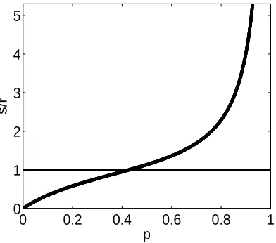
The boundary between the two behaviours in (p, s/r) parameter space is illustrated in figure 7. Since we require s > r, only the area s/r > 1 is relevant. In the majority of the region θr decreases with L as in Section 4.2; however, in the smaller region, for p
closer to unity and smaller s/r but still with s/r >1, we findθr increaseswith L.
5. Conclusion
0 0.2 0.4 0.6 0.8 1 0
1 2 3 4 5
p
[image:17.595.245.441.99.272.2]s/r
Figure 7. Illustration of the parameter space (p, s/r). In the region below and to the right of the thicker line (35), and above the thinner line, bothθrandθs increase with
L; above the solid line,θs increases andθr decreases with substrate length,L.
the shorter polymer yields the greatest total coverage as then the large polymers land frequently, quickly filling the binding sites early in the process, and later, when there is no room for long polymers to bind, the shorter polymers are able to fill in the gaps. In this manner, coverages of over 90% can be achieved. We define the R´enyi constant for shorter polymers by φr and that for longer polymers by φs, then if there is a small
probability of the shorter polymer binding, we rapidly find φs of the substrate covered,
leaving 1−φs vacant. Ifr ≪s, then over a longer timescale φr(1−φs) of the substrate
will be covered by the shorter polymer. This means the total coverage is φs+φr−φrφs.
If we take the R´enyi constant for the continuous system as a typical example, that is
φ=φr =φs = 0.7475979,then we find a total coverage of φ(2−φ) = 0.936.
We observe different asymptotic behaviour of coverages in the limit of large substrate lengths. In all cases, the total coverage and that of the longer polymer behave as in the one-component system, that is, as substrate length L increases, so does the coverage, approaching a constant as the substrate length, L → ∞, this limit
binding of the shorter polymer and where the ratio of polymer lengths is not too large, in which all coverages increase with substrate length. Asymptotic analysis of the system has revealed conditions on the parameters under which each form of limiting behaviour holds.
In future work it would be interesting to investigate the binding of mixtures on two-dimensional substrates, to see if such more general systems exhibit similar or a wider variety of behaviours in their large size limits.
Acknowledgements
The work of LR was supported by a Wellcome Trust Biomedical Vacation Scholarship (2014) for which we are grateful. We thank Laura Davis and Nathan Bishop for performing preliminary numerical simulations. We are also grateful to the referee for helpful suggestions.
References
[1] Adamcyk Z and Weronski P 1998 Random sequential adsorption on partially covered surfaces.J. Chem. Phys.1089851
[2] Baram A and Kutasov D 1992 Random sequential adsorption on a quasi-one-dimensional lattice: an exact solution.J. Phys. A: Math. Gen.25L493
[3] Bonnier B, Boyer D and Viot P 1994 Pair correlation function in random sequential adsorption processes.J. Phys. A; Math. Gen.273671–3682
[4] Burridge DJ and Mao Y 2004 Recursive approach to random sequential adsorptionPhys. Rev. E
69037102
[5] Cadilhe A, Ara´ujo NAM and Privman V 2007. Random sequential adsorption: from continuum to lattice and pre-patterned substrates.J. Phys.: Condens. Matter19065124
[6] Cornette V, Linares D, Ramirez-Pastor AJ and Nieto F 2007 Random sequential adsorption of polyatomic species.J. Phys. A: Math. Gen.4011765
[7] Dias CS, Ara´ujo, NAM, Cadilhe A 2012 Analytical and numerical study of particles with binary adsorption.Phys. Rev. E85041120
[8] Epstein IR 1979 Kinetics of large-ligand binding to one-dimensional lattices: theory of irreversible bindingBiopolymers 18765–804
[9] Evans JW 1993 Random and cooperative sequential adsorption.Rev. Mod. Phys. 651281–1329 [10] Feder J 1980 Random sequential adsorption.J. Theor. Biol.87237–254
[11] Flory P 1958 Intermolecular reaction between neighboring substituents of vinyl polymers.J. Am. Chem. Soc.611518–1521
[12] Grosberg AY, Nguyen TT and Shklovskii BI 2002 Colloquium: the physics of charge inversion in chemical and biological systems.Rev. Mod. Phys.74329–345
[13] Hassan MK and Kurths J 2001 Competitive random sequential adsorption of point and fixed-sized particles: analytical results.J. Phys. A: Math. Gen.34 7517
[14] Hassan MK, Schmidt J, Blasius B and Kurths J 2002 Jamming coverage in competitive random sequential adsorption of a binary mixture.Phys. Rev. E65045103(R)
[15] Hinrichsen EL, Feder J and Jøssang T 1986 Geometry of random sequential adsorption.J. Stat. Phys.44 793–827
[17] MacLeod AS and Gladden, LF 1999 The influence of the random sequential adsorption of binary mixtures on the kinetics of hydrocarbon hydrogenation reactions.J. Chem. Phys.1104000 [18] Maltsev E, Wattis JAD and Byrne HM 2006. DNA charge neutralisation by linear polymers:
irreversible binding.Phys. Rev. E74011904.
[19] Maltsev E, Wattis JAD and Byrne HM 2006 DNA charge neutralisation by linear polymers, II: reversible binding.Phys. Rev. E, 74041918
[20] McGhee JD and von Hippel PH 1974 Theoretical aspects of DNA-protein interactions: co-operative and non-co-operative binding of large ligands to a one-dimensional homogeneous lattice.J. Mol. Biol.86469–489
[21] Meyfroyt TMM, Borst SC, Boxman OJ, Denteneer, D 2014 A cooperative sequential adsorption model for wireless gossiping.arXiv:1407.6396
[22] Purves B, Reeve L, Wattis JAD, Mao Y 2015 Scaling behaviour near jamming in random sequential adsorption.Phys Rev E91022118.
[23] Porschke P 1984 Dynamics of DNA condensation.Biochemistry 234821–4828
[24] R´enyi A 1958 On a one-dimensional problem concerning random space-filling.Publ. Math. Inst. Hungar. Acad. Sci.,3109–127
[25] Talbot J and Schaaf P 1989 Random sequential adsorption of mixtures.Phys. Rev. A40, 422–427. [26] Tarjus G, Schaaf P, and Talbot J. 1990 Generalized random sequential adsorption.J Chem Phys
938352–8360
[27] Talbot J, Tarjus G, van Tassel PR and Viot P 2000 From car parking to protein adsorption: an overview of sequential adsorption processes.Coll & Surf A: Physicochem & Eng Aspects 165 287–324.