(will be inserted by the editor)
Exact Bayesian Inference for the Bingham Distribution
Christopher J. Fallaize · Theodore Kypraios
Received: date / Accepted: date
Abstract This paper is concerned with making Bayesian inference from data that are assumed to be drawn from a Bingham distribution. A barrier to the Bayesian ap-proach is the parameter-dependent normalising constant of the Bingham distribution, which, even when it can be evaluated or accurately approximated, would have to be calculated at each iteration of an MCMC scheme, thereby greatly increasing the computational burden. We propose a method which enables exact (in Monte Carlo sense) Bayesian inference for the unknown pa-rameters of the Bingham distribution by completely avoiding the need to evaluate this constant. We apply the method to simulated and real data, and illustrate that it is simpler to implement, faster, and performs better than an alternative algorithm that has recently been proposed in the literature
Keywords
1 Introduction
Observations that inherit a direction occur in many sci-entific disciplines (see, for example, Mardia and Jupp 2000). For example, directional data arise naturally in the biomedical field for protein structure (Boomsma
Christopher J. Fallaize·Theodore Kypraios
School of Mathematical Sciences, University Park,University of Nottingham
Nottingham, NG7 2RD, United Kingdom E-mail: [email protected]
S. Author second address
et al. 2008), cell–cycle (Rueda et al. 2009) and circa-dian clock experiments (Levine et al. 2002); see also the references in Ehler and Galanis (2011). A distri-bution that has proved useful as a model for spherical data which arise as unsigned directions is the Bingham distribution (Bingham 1974; Mardia and Jupp 2000).
The Bingham distribution can be constructed by conditioning a zero-mean multivariate Normal (MVN) distribution to lie on the sphereSq−1 of unit radius in
Rq. In particular, for a given matrix A of dimension q×q, the density with respect to the uniform measure onSq−1 is given by
f(x;A) = exp (−x TAx)
c(A) , x
Tx= 1 and x∈
Rq, (1)
wherec(A) is the corresponding normalising constant. Having observed some directional data, interest then lies in inference for the matrixAin (1). The likelihood of the observed data given the parameters can easily be written down and at first glance it appears that maximum likelihood inference forAis straightforward. However, inferring the matrix A is rather challenging. That is due to the fact that the likelihood of the ob-served data given the matrixAinvolves the parameter-dependent normalising constantc(A) which, in the gen-eral case, is not available in closed form. Therefore this poses significant challenges to undertake statistical in-ference involving the Bingham distribution either in a frequentist or Bayesian setting.
very little attention has been drawn in the literature concerning estimation of A within a Bayesian frame-work. Walker (2013) considered Bayesian inference for the Bingham distribution which removes the need to compute the normalising constant, using a (more gen-eral) method that was developed earlier (Walker 2011) and cleverly gets around the intractable nature of the normalising constant. However, it requires the intro-duction of several latent variables and a Reversible-Jump Markov Chain Monte Carlo (RJMCMC) sam-pling scheme.
The main contribution of this paper is to show how one can draw Bayesian inference for the matrixA, by exploiting the recent developments in Bayesian compu-tation for distributions with doubly intractable normal-ising constants (Møller et al. 2006; Murray et al. 2006). The main advantage of our approach is that it does not require any numerical approximation toc(A) and hence enablesexact(in the Monte Carlo sense) Bayesian infer-ence forA. Our method relies on being able to simulate exactsamples from the Bingham distribution which can be done by employing an efficient rejection sampling al-gorithm proposed by Kent et al. (2013).
The rest of the paper is structured as follows. In Section 2 we introduce the family of Angular Central Gaussian distributions and illustrate how such distribu-tions serve as efficient proposal densities to sample from the Bingham distribution. In Section 3 we describe our proposed algorithm while in Section 4 we illustrate our method both using simulated and real directional data from earthquakes in New Zealand. In Section 5 we dis-cuss the computational aspects of our method as well as directions for future research.
2 Rejection Sampling 2.1 Preliminaries
Rejection sampling (Ripley 1987) is a method for draw-ing independent samples from a distribution with prob-ability density functionf(x) =f∗
(x)/Zfassuming that we can evaluate f∗(x) for any value x, but may not necessarily knowZf. Suppose that there exists another distribution, with probability density function g(x) = g∗(x)/Z
g, often termed anenvelope density, from which we can easily draw independent samples and can evalu-ateg∗(x) at any valuex. We further assume that there
exists a constant M∗
for whichM∗ g∗
(x) ≥f∗ (x) ∀x. We can then draw samples fromf(x) as follows:
1. Draw a candidate value y from g(x) and u
from U(0,1);
2. if u≤ Mf∗∗g(y)∗(y) accept y; otherwise reject
y and go to step 1.
The set of accepted points provides a sample from the target densityf(x). It can be shown that the num-ber of trials until a candidate is accepted has a geomet-ric distribution with meanM, where
M = sup x∈R
f(x) g(x)
<∞. (2)
Therefore, the algorithm will work efficiently provided that M is small or, in other words, the probability of acceptance (1/M) is large. We should note that it is not necessary to know the normalising constants Zf and
Zg to implement the algorithm; the only requirement is being able to draw from the envelope density g(x) and knowledge of M∗
(rather than M which depends on the normalising constant of the likelihood function and cannot be computed).
2.2 The Angular Central Gaussian Distribution
The family of the angular central Gaussian(ACG) dis-tributions is an alternative to the family of the Bingham distributions for modelling antipodal symmetric direc-tional data (Tyler 1987). An angular central Gaussian distribution on the (q−1)−dimensional sphere Sq−1 can be obtained by projecting a multivariate Gaussian distribution in Rq, q ≥ 2, with mean zero onto Sq−1 with radius one. In other words, if the vector y has a multivariate Normal distribution in Rq with mean 0 and variance covariance matrix Ψ, then the vector x=y/||y|| follows an ACG distribution onSq−1 with
q×q symmetric positive−definite parameter matrixΨ (Mardia and Jupp 2000). The probability density func-tion of the ACG distribufunc-tion with respect to the surface measure onSq−1 is given by
g(x;Ψ) =w−1 q |Ψ|
−1/2 xTΨ−1x−q/2 =cACG(Ψ)g∗(x;Ψ)
where the constantwq = 2πq/2/Γ(q/2) represents the surface area onSq−1. Denote byc
2.3 Rejection Sampling for the Bingham Distribution
Kent et al. (2013) have demonstrated that one can draw samples from the Bingham distribution using the ACG distribution as an envelope density within a rejection sampling framework. In particular, they proposed the following algorithm to simulate a value from the Bing-ham distribution with parameter matrixA:
1. Set Ψ−1=I
q+2bA and M
∗≥sup
x
nf∗(x) g∗(x) o
;
2. draw u from U(0,1) and a candidate value y
from the ACG distribution on
the sphere with parameter matrix Ψ;
3. if u < f∗(y;A)
M∗g∗(y;Ψ) accept y; otherwise reject
y and go to Step 1.
Here, f∗(y;A) = exp(−yTAy) and
g∗(y;Ψ) = (yTΨ−1y)−q
2, the unnormalized Bingham
and ACG densities respectively, and b < q is a tun-ing constant. We found that setttun-ingb = 1 as a default works well in many situations, but an optimal value can be found numerically by maximising the acceptance probability 1/M (see, for example, Ganeiber 2012).
3 Bayesian Inference 3.1 Preliminaries
Consider the probability density function of the Bing-ham distribution as given in (1). If A=V ΛVT is the Singular Value Decomposition ofAwhereV is orthog-onal and Λ = diag(λ1, . . . , λq), then it can be shown that if x is drawn from a distribution with probabil-ity densprobabil-ity functionf(x;A), the corresponding random vector y = XTV is drawn from a distribution with density f(x;Λ) (see, for example, Kume and Walker 2006; Kume and Wood 2007). Therefore, without loss of generality, we assume thatA=Λ= diag(λ1, . . . , λq). Moreover, to ensure identifiability, we assume thatλ1≥
λ2≥. . . λq = 0 (Kent 1987). We discuss in Section 3.3 how one can draw inference for an arbitrary symmet-ric matrixAwhich may not necessarily be diagonal. In the case where A=Λthe probability density function becomes
f(x;Λ) = exp n
−Pqi=1−1λix2i o
c(Λ) (3)
with respect to a uniform measure on the sphere and
c(Λ) = Z
x∈Sq−1
exp (
−
q−1 X
i=1
λix2i )
dSq−1(x).
Suppose (x1,x2, . . . ,xn) is a sample of unit vectors in Sq−1 from the Bingham distribution with density (3). Then the likelihood function is given by
L(Λ) = 1 c(Λ)nexp
−
q−1 X
i=1
λi n X
j=1
xij 2
= 1
c(Λ)nexp (
−n
q−1 X
i=1
λiτi )
, (4)
where τi = 1nPni=1 xij 2
. The data can therefore be summarised by (n, τ1, . . . , τq−1), and (τ1, . . . , τq−1) are sufficient statistics for (λ1, . . . , λq−1).
3.2 Bayesian Inference
We are interested in drawing Bayesian inference for the matrixΛ, or equivalently, for λ = (λ1, . . . , λq−1). The likelihood function in (4) reveals that the normalising constant c(Λ) plays a crucial role. The fact that there does not exist a closed form expression forc(Λ) makes Bayesian inference forΛvery challenging.
For example, if we assign independent Exponential prior distributions to the elements ofλwith rateµi(i.e. mean 1/µi) subject to the constraint thatλ1 ≥ λ2 ≥
. . .≥λq−1then the density of the posterior distribution ofΛup to proportionality given the data is as follows:
π(λ|x1, . . . ,xn)∝L(Λ) q−1 Y
i=1
exp{−λiµi}
×1(λ1≥λ2≥. . .≥λq−1)
= 1
c(Λ)n exp (
−
q−1 X
i=1
λi(nτi+µi) )
×1(λ1≥λ2≥. . .≥λq−1). (5) Consider the following Metropolis-Hastings algorithm which aims to draw samples fromπ(λ|x1, . . . ,xn):
1. Suppose that the current state of the chain
is λcur;
2. Update λ using, for example, a random walk
Metropolis step by
proposing λcan∼Nq−1(λcur, Σ);
Note thatNq−1(m, S) denotes the density of a mul-tivariate Normal distribution with mean vectormand variance-covariance matrixS. Step 2 of the above algo-rithm requires the evaluation of the ratio π(λcan|x1, . . . ,xn)/π(λcur|x1, . . . ,xn), which in turn involves evaluation of the ratioc(Λcan)/c(Λcur). There-fore, implementing the above algorithm requires an ap-proximation of the normalising constant. In principle, one can employ one of the proposed methods in the literature which are based either on asymptotic expan-sions (Kent 1987), saddlepoint approximations (Kume and Wood 2005) or holonomic gradient methods (Sei and Kume 2013). Although such an approach is feasi-ble, in practice, it can be very computationally costly since the normalising constant would have to be approx-imated at every single MCMC iteration. Furthermore, despite how accurate these approximations may be, the stationary distribution of such an MCMC algorithm won’t be the distribution of interest π(λ|x1, . . . ,xn), but an approximation to it.
3.2.1 An Exchange Algorithm
The main contribution of this paper is to demonstrate that recent developments in Markov Chain Monte Carlo algorithms for the so-called doubly intractable distribu-tions enable drawing exact Bayesian inference for the Bingham distribution without having to resort to any kind of approximations.
Møller et al. (2006) proposed an auxiliary variable MCMC algorithm to sample from doubly intractable distributions by introducing cleverly chosen variables in to the Metropolis-Hastings (M-H) algorithm such that the normalising constants cancel in the M-H ratio. Con-sider augmenting the observed data x with auxiliary datay, which has the same state space asx, leading to the joint distribution
π(y,x,λ) =π(y|x,λ)π(x,λ),
where π(x,λ) =f(x|λ)π(λ)∝π(λ|x), the target pos-terior distribution of interest. There is freedom of choice in the conditional densityπ(y|x,λ). For example, this could be the same density as that of the datax, evalu-ated at some fixed value ofλ, ˆλsay. This would require a good representative value of λ, obtained for exam-ple from a pseudo-likelihood estimator, for good per-formance. Note also that it is necessary to store values of the auxiliary variables from one iteration to the next.
A simpler version that avoids having to specify the conditional density of the auxiliary variables was pro-posed in Murray et al. (2006). Although both approaches rely on being able to simulate realisations from the Bingham distribution (see Section 2.3), we choose to adapt to our context the approach presented in Murray et al. (2006) because it is simple and easy to implement, since a value of the parameter of interest does not need to be specified. Proposalsλ′ are drawn from a density h(·|λ), although in general this density does not have to depend on the current state ofλ. For example, random walk proposals centred at λ or independence sampler proposals could be used. The algorithm proceeds as fol-lows:
1. Draw λ′ ∼h(·|λ)
;
2. Draw y∼f(·|λ′)
;
3. Accept the move from λ to λ′
with probability
min
1,f
∗(x|λ′)π(λ′)h(λ|λ′)f∗(y|λ) f∗(x|λ)π(λ)h(λ′|λ)f∗(y|λ′) ×
c(Λ)c(Λ′) c(Λ)c(Λ′)
,
wheref∗(x;A) = exp(−xTAx) is the unnormalized Bingham density as previously and f is the normal-ized density. Under this scheme, the marginal distribu-tion of λ is the target posterior distribution of inter-est, but crucially, note that all intractable normalising constants cancel above and below the fraction. Hence, the acceptance probability can be evaluated, unlike in the case of a standard Metropolis-Hastings scheme. We are thus able to draw samples from our target posterior distribution, provided we can simulate exactly from the Bingham distribution. The exchange move can be inter-preted as offering the observed dataxto the proposed parameterλ′ and similarly to offer the auxiliary data ythe parameterλ.
This algorithm, due to Murray et al. (2006), is a spe-cial case of a more general algorithm which draws two sets of new auxiliary variablesyandy′
at each iteration (Storvik 2011). It is the special case where only propos-als such thaty=y′
3.3 Bayesian Inference for an Arbitrary Symmetric MatrixA
Following Walker (2013) we have thus far assumed that the matrixAin Equation 1 is diagonal. However, when dealing with real datasets this may not necessarily the case. Therefore, we now describe how to draw Bayesian inference for a general symmetric matrixA, given data x1, . . . ,xnwhich are drawn from the corresponding Bing-ham distribution.
Denote by aij the elements of (the random) ma-trixAwhereaij =ajifori, j= 1, . . . , q. The likelihood function is given byL(A) = exp (−Pni=1xiTAxi)/c(A)n. We assign independent Normal prior distributions to each aij fori ≥j with mean zero and variance v and hence the posterior distribution has density propor-tional to
exp
−Pni=1xTi Axi exp−2v1aTa
c(A)n , (6)
where a = (a1, . . . , ana) is the vector of distinct ele-ments ofA, of which there arena=q+
q 2
!
.
To perform inference forA, based on a sample ofn points assumed to be from a Bingham distribution, we can again apply the exchange algorithm. Suppose the current value ofAisAcur, with elementsacur. We first propose a move to a candidate value ofA,Acan (with elements acan) , drawn from some density h(·|Acur). We then sample auxiliary datay, by sampling ndata points from the Bingham density (1) with parameter Acan. In this paper, we use random walk Metropolis updates forA, by drawing candidate values for the ele-ments ofAcan from a multivariate normal distribution with mean vectoracur and covariance matrixσ2
aI. We find this satisfactory for our work here, but more elab-orate proposals could be constructed, such as an inde-pendence sampler which draws candidate values from a good approximation to the posterior distribution of A; we do not consider such proposals further in this paper. In the general case, we can writeA=V ΛVT, where
Λ is the diagonal matrix of parameter values consid-ered previously, and V is an orthogonal matrix. Thus, inference forΛcan be performed by decomposing each sampled value of A in this manner, but we now also obtain posterior samples for the orthogonal component V. (Previously, whenAwas assumed to be diagonal, we simply hadV =I.) Again, for identifiability, we apply the constraintλ1≥λ2≥. . .≥λq = 0.
3.3.1 Example
To illustrate inference for generalA, we apply our method to the data of Bingham (1974). The data consist of n= 150 measurements of a certain axis of interest re-lating to calcite grains from the Taconic Mountains of New York state, and yield a moment of inertia (or sum of squares and products) matrix
T = 150 X
i=1
xixTi =
76.5575 18.2147 12.2406 18.2147 46.7740 6.8589 12.2406 6.8589 26.6670
.
We used the settingsv = 100 andσ2
a = 0.04, and base inference on a sample ofN = 100000 values from the posterior distribution (6). This value ofσ2
a was found by experimentation to result in good mixing properties for the chain in this example, and alteringσ2
a can affect the mixing and increase autocorrelation in the chain. As mentioned previously, more elaborate proposals could be constructed, but this is not pursued further here. For the diagonal componentΛ, we obtain posterior median valuesλ1= 3.631 andλ2= 1.963, compared with maxi-mum likelihood estimates of ˆλ1= 3.518 and ˆλ2= 1.956. For the orthogonal component of A, we have samples V1, . . . , VN, obtained from the spectral decomposition of each sampled matrix Ai, i = 1, . . . , N. To obtain a summary value, we first form the element-wise sample
mean ofV, ¯V =N1 N X
i=1
Vi. We then decompose this into
¯
V = ˆV K, where K = ( ¯VTV¯)1/2, the positive definite square root of ¯VTV¯, and ˆV is an orthogonal matrix known as the polar part of ¯V (Mardia and Jupp 2000);
ˆ
V is then our estimate of the orthogonal componentV. We obtain
ˆ V =
0.1795 −0.4404 0.8797 0.1394 0.8966 0.4204
−0.9738 0.0472 0.2223
.
The corresponding maximum likelihood estimate is
−0.1723 −0.4439 0.8794
−0.1516 0.8940 0.4216 0.9733 0.0606 0.2213
4 Applications 4.1 Artificial Data
We illustrate the proposed algorithm to sample from the posterior distribution ofλusing artificial data.
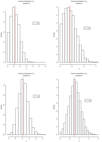
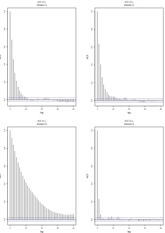
Dataset 1 Consider a sample of n= 100 unit vectors (x1, . . . ,x100) which result in the pair of sufficient statis-tics (τ1, τ2) = (0.30,0.32). We assign independent Ex-ponential prior distributions with rate 0.01 (i.e. mean 100) to the parameters of interestλ1 andλ2subject to the constraint thatλ1 ≥λ2; note that we also implic-itly assume that λ1 ≥λ2 ≥λ3 = 0. We implemented the algorithm which was described in Section 3.2.1. The parameters were updated in blocks by proposing a can-didate vector from a bivariate Normal distribution with mean the current values of the parameters and variance-covariance matrixσI, whereIis the identity matrix and the samples were thinned, keeping every 10th value. Convergence was assessed by visual inspection of the Markov chains and we found that by using σ= 1 the mixing was good and achieved an acceptance rate be-tween 25% and 30%. Figure 1 shows a scatter plot of the sample from the joint posterior distribution (left panel) whilst the marginal posterior densities forλ1andλ2are shown in the top row of Figure 2. The autocorrelation function (ACF) plots, shown in the top row of Figure 3, reveal good mixing properties of the MCMC algorithm and (by visual inspection) appear to be much better than those shown in Walker (2013, Figure 1). Mardia and Zemroch (1977) report maximum likelihood esti-mates of ˆλ1 = 0.588, ˆλ2 = 0.421, with which our re-sults broadly agree. Although in principle one can de-rive (approximate) confidence intervals based on some regularity conditions upon which it can be proved that the MLEs are (asymptotically) Normally distributed, an advantage of our (Bayesian) approach is that it al-lows quantification of the uncertainty of the parameters of interest in a probabilistic manner.
Dataset 2 We now consider an artificial dataset of 100 vectors which result in the pair of sufficient statistics (τ1, τ2) = (0.02,0.40) for which the maximum likeli-hood estimates are ˆλ1= 25.31, ˆλ2= 0.762 as reported by Mardia and Zemroch (1977). We implement the pro-posed algorithm by assigning the same prior distribu-tions toλ1andλ2as for Dataset 1. A scatter plot of a sample from the joint posterior distribution is shown in
Figure 1 (right panel), showing that our approach gives results which are consistent with the MLEs. Marginal posterior densities forλ1 andλ2are shown in the bot-tom row of Figure 2, and ACF plots are shown in the bottom row of Figure 3. This example shows that our al-gorithm performs well whenλ1>> λ2 as well as when the difference between λ1 and λ2 is much smaller, as was the case in Dataset 1.
4.2 Earthquake data
As an illustration of an application to real data, we con-sider an analysis of earthquake data recently analysed by Arnold and Jupp (2013). An earthquake gives rise to three orthogonal axes, and geophysicists are inter-ested in analysing such data in order to compare earth-quakes at different locations and/or at different times. An earthquake gives rise to a pair of orthogonal axes, known as the compressional (P) and tensional (T) axes, from which a third axis, known as the null (B) axis is obtained viaB=P×T. (Arnold and Jupp (2013) label this theAaxis, but we have used Afor the parameter of the Bingham distribution.) Each of these quantities are determined only up to sign, and so models for axial data are appropriate. The data can be treated as or-thogonal axial 3-frames inR3and analysed accordingly, as in Arnold and Jupp (2013), but we will illustrate our method using theBaxes only. In general, an orthogonal axialr-frame inRp, r≤p, is an ordered set of raxes,
{±u1, . . . ,±ur}, whereu1, . . . , urare orthonormal vec-tors inRp(Arnold and Jupp 2013). The familiar case of data on the sphereS2 is the special case corresponding top= 3, r= 1, which is the case we consider here.
0.0 0.5 1.0 1.5 2.0 2.5 3.0
0.0
0.5
1.0
1.5
Posterior Sample of (λ1,λ2)
(Dataset 1)
λ1
λ2
15 20 25 30 35 40
0.0
0.5
1.0
1.5
2.0
Posterior Sample of (λ1,λ2)
(Dataset 2)
λ1
λ2
Fig. 1 Sample from the joint posterior distribution of λ1 andλ2 for Dataset 1 (left) and Dataset 2 (right) as described in
Section 4.
our method by fitting Bingham models to the B axes from each of the individual clusters and considering the posterior distributions of the parameters of the diago-nal component of the Bingham parameter matrix. We will denote these parameters from the CCA, CCB and SI models asλA
i ,λBi andλSi respectively,i= 1,2. The observations for the two clusters of observa-tions near Christchurch yield sample data of (τA
1, τ2A) = (0.1152360,0.1571938) for CCA and (τB
1 , τ2B) = (0.1127693,0.1987671) for CCB. The data
for the South Island observations are
(τS
1, τ2S) = (0.2288201,0.3035098). We fit each dataset separately by implementing the proposed algorithm. Exponential prior distributions to all parameters of in-terest (mean 100) were assigned, subject to the con-straint thatλj1≥λ
j
2 forj=A, B, S. Scatter plots from the joint posterior distributions of the parameters from each individual analysis are shown in Figure 4. The plots for CCA and CCB look fairly similar, although λ2is a little lower for the CCB cluster. The plot for SI cluster suggests that these data are somewhat different.
To establish more formally if there is any evidence of a difference between the two Christchurch clusters, we consider the bivariate quantity (λA
1−λB1, λA2−λB2).If there is no difference between the two clusters, then this quantity should be (0,0). In Figure 5 (left panel), we show the posterior sample of this quantity, and a 95% probability region obtained by fitting a bivariate normal distribution with parameters estimated from this sam-ple. The origin is contained comfortably within this re-gion, suggesting there is no real evidence for a difference between the two clusters. Arnold and Jupp (2013) ob-tained ap-value of 0.890 from a test of equality for the two populations based on treating the data as full ax-ial frames, and our analysis on theB axes alone agrees with this.
The right panel of Figure 5 shows a similar plot for the quantity (λA
[image:7.612.62.512.36.357.2]popu-Posterior Distribution of λ1
(Dataset 1)
λ1
Density
0.0 0.5 1.0 1.5 2.0 2.5 3.0
0.0
0.2
0.4
0.6
0.8
1.0
MLE
Posterior Distribution of λ2
(Dataset 1)
λ2
Density
0.0 0.5 1.0 1.5
0.0
0.2
0.4
0.6
0.8
1.0
1.2
1.4
MLE
Posterior Distribution of λ1
(Dataset 2)
λ1
Density
15 20 25 30 35 40
0.00
0.02
0.04
0.06
0.08
0.10
MLE
Posterior Distribution of λ2
(Dataset 2)
λ2
Density
0.0 0.5 1.0 1.5 2.0
0.0
0.2
0.4
0.6
0.8
1.0
1.2
1.4
MLE
Fig. 2 Marginal posterior densities forλ1 andλ2 for Dataset 1 (top) and Dataset 2 (bottom) in Section 4.
lations, so again our analysis on the A axes agrees with this.
4.2.1 Inference for fullA
As well as testing for differences between the samples, it is of interest to determine whether theBaxes are verti-cal, since the observedP andT axes lie approximately in the horizontal plane. For the CCA cluster, our anal-ysis yields an estimate of the dominant eigenvector of
[image:8.612.113.461.40.522.2]0 10 20 30 40
0.0
0.2
0.4
0.6
0.8
1.0
lag
A
CF
ACF of λ1
(Dataset 1)
0 10 20 30 40
0.0
0.2
0.4
0.6
0.8
1.0
lag
A
CF
ACF of λ2
(Dataset 1)
0 10 20 30 40
0.0
0.2
0.4
0.6
0.8
1.0
lag
A
CF
ACF of λ1
(Dataset 2)
0 10 20 30 40
0.0
0.2
0.4
0.6
0.8
1.0
lag
A
CF
ACF of λ2
(Dataset 2)
Fig. 3 ACFs forλ1andλ2 for Dataset 1 (top) and Dataset 2 (bottom) in Section 4.
5 Discussion
There is a growing area of applications that require in-ference over doubly intractable distributions including directional statistics, social networks (Caimo and Friel 2011), latent Markov random fields (Everitt 2012), and large–scale spatial statistics (Aune et al. 2012) to name but a few. Most conventional inferential methods for such problems relied on approximating the
[image:9.612.117.457.41.521.2]con-3 4 5 6 7 8
2
3
4
5
6
Posterior Sample of (λ1
A,λ
2
A)
λ1 A
λ2
A
2 4 6 8 10
1
2
3
4
5
Posterior Sample of (λ1
B,λ
2
B)
λ1 B
λ2
B
0 1 2 3 4 5
0.0
0.5
1.0
1.5
2.0
2.5
3.0
Posterior Sample of (λ1
S,λ
2
S)
λ1 S
λ2
S
Fig. 4 Posterior samples for differences in λ1 and λ2 for the two sets of Christchurch data (left) and South Island and
Christchurch data A (right). This shows a clear difference between the South Island and Christchurch data, but suggests no difference between the two sets of Christchurch data.
−4 −2 0 2 4 6
−2
−1
0
1
2
3
4
CCA−CCB
λ1
A− λ
1 B
λ2 A−
λ2
B
−8 −6 −4 −2 0
−5
−4
−3
−2
−1
0
1
SI−CCB
λ1
S− λ
1 B
λ2 S−
λ2
B
Fig. 5 Posterior samples for differences in λ1 and λ2 for the two sets of Christchurch data (left) and South Island and
[image:10.612.66.508.43.239.2] [image:10.612.61.508.305.620.2]stant became available; see Møller et al. (2006); Murray et al. (2006); Walker (2011); Girolami et al. (2013).
In this paper we were concerned with exact Bayesian inference for the Bingham distribution which has been a difficult task so far. We proposed an MCMC algorithm which allows us to draw samples from the posterior dis-tribution of interest without having to approximate this constant. We have shown that the MCMC scheme is i) fairly straightforward to implement, ii) mixes very well in a relatively short number of sweeps and iii) does not require the specification of good guesses of the unknown parameters. We have applied our method to both real and simulated data, and showed that the results agree with maximum likelihood estimates for the parameters. However, we believe that a fully Bayesian approach has the benefit of providing an honest assessment of the uncertainty of the parameter estimates and allows exploration of any non-linear correlations between the parameters of interest. In comparison to the approach recently proposed by Walker (2013) (which also avoids approximating the normalising constant) we argue that our algorithm is easier to implement, runs faster and the Markov chains appear to mix better.
In terms of computational aspects, our algorithm is not computationally intensive and this is particularly true for the number of dimensions that are commonly met in practice (e.g. q = 3). For all the results pre-sented here, we ran our MCMC chains for 106 itera-tions for each of the simulated and real data examples, which we found to be sufficient for good mixing in all cases. Our method was implemented in C++ and each example took between 20 and 30 seconds on a desktop PC with 3.1GHz processor1; note, that is considerably faster than the algorithm proposed by Walker (2013) in which “running 105iterations takes a matter of minutes on a standard laptop”. In general the time taken for our proposed algorithm will depend on the number of auxil-iary data pointsnthat need to be simulated, as well as the efficiency of the underlying rejection algorithm for the particular parameter values at each iteration. In ad-dition, the efficiency of the rejection algorithm is likely to deteriorate as the dimension q increases. In partic-ular, we found when we varied q from 3 to 7 that the probability of acceptance in the rejection sampling step was around 78%, 45%, 30%, 18% and 10% respectively. These numbers reveal why we found our algorithm to be very efficient for all our examples and efficient for at
1 Our code is available upon request.
least a moderate number of dimensions. However, we anticipate that it will become slower (in CPU time) for q≥7.
In both the simulated and real datasets we chose the proposal distribution h(λ′|λ) to be a multivari-ate Normal distribution with mean the current value of the chain and variance covariance matrix equal to σI. Any drawn values which did not satisfy the con-straint λ1 > . . . > λq−1 were rejected straight away. The probability of the constraint being satisfied will decrease with q and in consequence such a proposal will become very inefficient for large values ofq. There-fore, we have also implemented an alternative proposal distribution in which the constraint is implicitly taken account. Consider for illustration the case whereq= 3; we drawλ′2from a Normal distribution centered at the current value ofλ2 and then we drawλ
′
1 from a (trun-cated) Normal distribution with meanλ1subject to the constraint thatλ′1> λ
′
2. It is easy to see how such a pro-posal can be generalised forq >3. We have performed simulation studies (results not shown) and found that such a proposal distribution is more efficient than the standard random walk Metropolis when q and/or the difference between the successive values of the eigen-valueλ,i= 1, . . . , q−1 is large.
With regards to the choice of prior distributions we assigned independent Exponential distributions with rate µ to eachλi, i = 1, . . . q−1 and independent Normal distributions with mean zero and variancev for the el-ements ofA. We have used largely uninformative prior distributions in all applications and in particular we choseµ = 10−2 and v = 102. However, we performed some prior sensitivity analysis by choosing different val-ues for both hyperparameters, e.g. 10−3 and 10−1 for
µ and 10 and 103 for v and we found that there no material change in the inferred posterior distributions. Statistical inference, in general, is not limited to parameter estimation. Therefore, a possible direction for future research within this context is to develop methodology to enable calculation of the model evi-dence (marginal likelihood). This quantity is vital in Bayesian model choice and knowledge of it will allow a formal comparison between competing models for a given dataset such as the application presented in Sec-tion 4.2.
mo-ments of the Bingham distribution. Finally, we would like to thank Ian Dryden for commenting on an earlier draft of this manuscript.
References
R Arnold and P E Jupp. Statistics of orthogonal axial frames.
Biometrika, 100(3):571–586, 2013.
Erlend Aune, Daniel P Simpson, and Jo Eidsvik. Parame-ter estimation in high dimensional gaussian distributions.
Statistics and Computing, pages 1–17, 2012.
Christopher Bingham. An antipodally symmetric distribution on the sphere. Ann. Statist., 2:1201–1225, 1974. ISSN 0090-5364.
W. Boomsma, K.V. Mardia, C.C. Taylor, J. Ferkinghoff-Borg, A. Krogh, and T. Hamelryck. A generative, probabilistic model of local protein structure. Proc Natl Acad Sci U S A, 105(26):8932–7, 2008.
Alberto Caimo and Nial Friel. Bayesian inference for ex-ponential random graph models. Social Networks, 33(1): 41–55, 2011.
Martin Ehler and Jennifer Galanis. Frame theory in direc-tional statistics. Statistics and Probability Letters, 81(8): 1046–1051, 2011.
Richard G Everitt. Bayesian parameter estimation for la-tent markov random fields and social networks. Journal of Computational and Graphical Statistics, 21(4):940–960, 2012.
Asaad M. Ganeiber. Estimation and simulation in directional and statistical shape models. PhD thesis, University of Leeds, 2012.
Mark Girolami, Anne-Marie Lyne, Heiko Strathmann, Daniel Simpson, and Yves Atchade. Playing russian roulette with intractable likelihoods. ArXiv preprint; arXiv:1306.4032, 2013.
John T. Kent. Asymptotic expansions for the Bingham dis-tribution. J. Roy. Statist. Soc. Ser. C, 36(2):139–144, 1987. ISSN 0035-9254. doi: 10.2307/2347545. URL http://dx.doi.org/10.2307/2347545.
John T. Kent, Asaad M. Ganeiber, and Kanti V. Mardia. A new method to simulate the Bingham and related dis-tributions in directional data analysis with applications.
ArXiv Preprint, 2013. http://arxiv.org/abs/1310.8110. A. Kume and Andrew T. A. Wood. Saddlepoint
ap-proximations for the Bingham and Fisher-Bingham nor-malising constants. Biometrika, 92(2):465–476, 2005. ISSN 0006-3444. doi: 10.1093/biomet/92.2.465. URL http://dx.doi.org/10.1093/biomet/92.2.465.
A. Kume and Andrew T. A. Wood. On the deriva-tives of the normalising constant of the Bingham dis-tribution. Statist. Probab. Lett., 77(8):832–837, 2007. ISSN 0167-7152. doi: 10.1016/j.spl.2006.12.003. URL http://dx.doi.org/10.1016/j.spl.2006.12.003.
Alfred Kume and Stephen G. Walker. Sampling from compositional and directional distributions.
Stat. Comput., 16(3):261–265, 2006. ISSN 0960-3174. doi: 10.1007/s11222-006-8077-9. URL http://dx.doi.org/10.1007/s11222-006-8077-9.
Joel D Levine, Pablo Funes, Harold B Dowse, and Jeffrey C Hall. Resetting the circadian clock by social experience in drosophila melanogaster. Science Signaling, 298(5600): 2010–2012, 2002.
K V Mardia and P J Zemroch. Table of maximum likelihood estimates for the bingham distribution. Statist. Comput. Simul., 6:29–34, 1977.
Kanti V. Mardia and Peter E. Jupp. Directional statistics. Wiley Series in Probability and Statistics. John Wiley & Sons Ltd., Chichester, 2000. ISBN 0-471-95333-4. Re-vised reprint of ıt Statistics of directional data by Mardia [ MR0336854 (49 #1627)].
J. Møller, A. N. Pettitt, R. Reeves, and K. K. Berthelsen. An efficient Markov chain Monte Carlo method for distributions with intractable normalising constants. Biometrika, 93(2):451–458, 2006. ISSN 0006-3444. doi: 10.1093/biomet/93.2.451. URL http://dx.doi.org/10.1093/biomet/93.2.451.
Iain Murray, Zoubin Ghahramani, and David J. C. MacKay. MCMC for doubly-intractable distributions. In Proceed-ings of the 22nd Annual Conference on Uncertainty in Ar-tificial Intelligence (UAI-06), pages 359–366. AUAI Press, 2006.
Brian D. Ripley.Stochastic simulation. Wiley Series in Prob-ability and Mathematical Statistics: Applied ProbProb-ability and Statistics. John Wiley & Sons Inc., New York, 1987. ISBN 0-471-81884-4. doi: 10.1002/9780470316726. URL http://dx.doi.org/10.1002/9780470316726.
Cristina Rueda, Miguel A. Fern´andez, and Shyamal Das Peddada. Estimation of parameters subject to or-der restrictions on a circle with application to es-timation of phase angles of cell cycle genes. J. Amer. Statist. Assoc., 104(485):338–347, 2009. ISSN 0162-1459. doi: 10.1198/jasa.2009.0120. URL http://dx.doi.org/10.1198/jasa.2009.0120.
Tomonari Sei and Alfred Kume. Calculating the nor-malising constant of the bingham distribution on the sphere using the holonomic gradient method.
Statistics and Computing, pages 1–12, 2013. ISSN 0960-3174. doi: 10.1007/s11222-013-9434-0. URL http://dx.doi.org/10.1007/s11222-013-9434-0.
Geir Storvik. On the flexibility of metropolishast-ings acceptance probabilities in auxiliary vari-able proposal generation. Scandinavian Journal of Statistics, 38(2):342–358, 2011. ISSN 1467-9469. doi: 10.1111/j.1467-9469.2010.00709.x. URL http://dx.doi.org/10.1111/j.1467-9469.2010.00709.x. David E. Tyler. Statistical analysis for the
angu-lar central Gaussian distribution on the sphere.
Biometrika, 74(3):579–589, 1987. ISSN 0006-3444. doi: 10.1093/biomet/74.3.579. URL http://dx.doi.org/10.1093/biomet/74.3.579.
Stephen G. Walker. Posterior sampling when the nor-malizing constant is unknown. Comm. Statist. Sim-ulation Comput., 40(5):784–792, 2011. ISSN 0361-0918. doi: 10.1080/03610918.2011.555042. URL http://dx.doi.org/10.1080/03610918.2011.555042. Stephen G. Walker. Bayesian estimation of the Bingham