A 3D Scene Analysis Framework and Descriptors for Risk Evaluation
R. Dupre, V. Argyriou, D. Greenhill
Kingston University
G. Tzimiropoulos
University Nottingham
Abstract
In this paper we evaluate the notion of scene analysis with regard to risk. We consider the problem of evaluat-ing risk and potential hazards in an environment and pro-viding a quantified risk score. A definition of risk is given incorporating two elements; Firstly scene stability, where Newtonian Physics are introduced into the scene analysis process, evaluating object stability within a scene. The ef-fectiveness of which is demonstrated by conducting experi-ments on several scenes including a variety of stability lev-els. Secondly the analysis of the intrinsic risk related prop-erties of an object, which is estimated using learning tech-niques and the utilisation of the 3D Voxel HOG descriptor, analysed against the state-of-the-art descriptors. Finally a new dataset is provided that is designed for scene analysis focusing on risk evaluation.
1. Introduction
Scene analysis is a research area covering a large range of topics with applications in traffic analysis [4], domestic robotics [32], and smart homes [5] amongst many others. In this work we consider one such topic; scene analysis with regard to risk, with the aim of providing a quantified risk score for a given three dimensional scene. To achieve this a system is proposed that will, through a combination of novel feature selection mechanisms and Newtonian physics, analyse the potential risk in a given 3D scene.
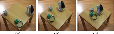
[image:1.612.311.543.215.398.2]The definition of what can be considered a risk or haz-ard in an environment is contextual. However reghaz-ardless of context, the elements that might contribute to the concept of risk can be broken down into components from which a decision can be made. These components include ele-ments such as shape, material, temperature, position and many others. For this work we propose a system which focuses on two of these elements; firstly object and scene stability, derived from the resultant energy outputs due to an applied force, as well as its subsequent effect on other objects within a scene. This is analysed using a novel com-bination of vision based and physics simulation techniques.
Figure 1: Example Scenes of objects with a variety of (top) haz-ardous properties (e.g. sharp, pointed) and (bottom) levels of sta-bility.
As an example consider the difference between a glass bot-tle placed at the corner of a table, against it being placed at the centre (Figure1).
Secondly, determining the intrinsic shape structures of an object which may add to the prospective hazard. To for-mulate this definition a voxel based three dimensional de-scriptor has been uterlised that is based on the principles of Histogram of Oriented Gradients. The proposed 3D Voxel HOG (3D VHOG) descriptor tries to identify dangerous el-ements or characteristics of an object (e.g. ‘hazardous fea-tures’). When combined with a boosting technique (Ad-aboost [12]), the resultant model aims to specify whether an object affects the potential risk in a given 3D scene (Figure
1). Importantly object recognition is not the goal, allow-ing the proposed approach to be more general and operate at a lower level. In object recognition a ‘feature’ is defined in terms of a specific structure in the data. Here the term ‘feature’ relates to an actual physical property of an object. In this work we define ‘hazardous features’ as any structure present in an object within the 3D scene that could increase risk (e.g. a knife’s blade being sharp/pointed).
In this paper we evaluate the concept of risk estimation in static and dynamic scenes by combining the novel use
2015 International Conference on 3D Vision
2015 International Conference on 3D Vision
of Newtonian physics mechanics and the introduction of a new feature descriptor. We define risk as a function of scene stability and the intrinsic properties of the present objects. Furthermore a novel dataset for 3D scene analysis was col-lected and will be available online.
The paper will continue as follows; in section 2 an anal-ysis of the similar areas of research and related work. The proposed methodologies and processes used in the work will be presented in section 3. Section 4 will outline the experiment environments and analyse the results. Finally, in section 5 conclusions are drawn.
2. Related Work
2.1. Scene Analysis and Risk Assessment
To date very little research has been done in automated risk analysis systems. [31,2] analyse indoor fall assessment for elderly adults; however in both proposed methods focus is given to analysing the person not the risk of the environ-ment. [37] introduces the notion of analysing the fall po-tential of objects in a scene given the influence of environ-mental events such as human intervention or earthquakes. However the interaction of objects is not considered nor is the potential risk of the object itself.
Another emerging area of research within 3D scene anal-ysis relates to Volumetric Reasoning. Here the applica-tion of logic based algorithms to existing object clusters is used to improve segmentation and clustering accuracy. [38] utilises the notion that clusters in a scene should be in a state of rest when simulation techniques are applied. Thus by using an iterative process clusters are grouped until such time as the scene is at equilibrium. [15] proposes a method that better fits bounding shapes to RGB-D clusters based on the premise that a good 3D representation of a scene is sta-ble, fits the data well and is self-supporting. Battaglia [1] introduces the idea of a ‘intuitive physics engine (IPE)’ that tries to mimic a humans cognitive simulation process when analysing a scene. It is also worth mentioning the follow-ing papers that consider similar concepts and approaches for scene analysis [22,11,18,20,21,9,19,8].
Although the concept of risk evaluation is raised in some of this work, an automated form of risk evaluation for a given scene is not fully addressed.
2.2. Object Retrieval and Scene Descriptors
Object retrieval and feature selection are research sub-jects that have received a huge amount of work in recent years. The initial concept of HOG features [6] revolution-ized the 2D object recognition world by creating a local descriptor that was resistant to geometric and photometric changes. Onishi [24] uses HOG on images from a monoc-ular camera system to recognise human posture in a scene and estimate, using regression, the joint angles on a 3D
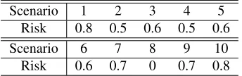
hu-Figure 2: Example of the acquisition process using Kinect Fusion and some of the obtained 3D scenes.
Pre-Processing
Stability Estimation
Hazard Features
Estimation 3D Voxel HOG Descriptor
Risk Value Input: 3D Scene
with Kinect Fusion
Figure 3: An overview of the proposed risk assessment framework.
man model. Buch in [3] implements a vehicle recognition framework, using a patch definition system on a 3D repre-sentation of the found vehicle, combined with a traditional two dimensional implementation of the HOG descriptor.
[image:2.612.310.546.73.332.2]3D Scene Capturing e.g. Kinect Fusion
Plane removal Voxelization Segmentation & Bounding Boxes
[image:3.612.51.289.72.164.2]Pre-Processing
Figure 4: An overview of the pre processing stage.
3. Proposed Methodology
The following section will discuss the proposed method-ologies used to define a weighted risk estimation model, and how the parameters in that model are established from a 3D scene. An overview of this framework is shown in Figure3.
3.1. Pre Processing
Before the risk in a scene can be evaluated, pre pro-cessing steps are required to convert the input data, a mesh model of the scene, into a usable format (Figure 4). The scene data and 3D mesh model reconstruction of an envi-ronment is acquired using Kinect Fusion [14] (Figure2). Alternatively other multi-camera acquisition systems [35] or sensors (e.g. thermal or acoustic cameras) could be used. The surface on which the objects are set requires removal to aid with clustering, the work in [34] provides solutions for these problems. The removed plane’s dimensions will later be used to define the surface during simulation.
Voxels are defined along the faces of the scene’s 3D mesh, voxels enclosed within a mesh are also classified as part of the scene allowing us to consider features based on an objects’ density. This resultant volume represents a bi-nary classification of either object or not. With this clas-sification in place, clustering of the voxel volume can be applied grouping voxels into object clusters. A number of different clustering algorithms were tested, using modified versions of the work presented in [34,7]. A range of other clustering algorithms were also considered. A bounding box for each object cluster is defined (Figure4right), with the number of voxels within that bounding box counted and used as a rudimentary measure of mass. For the purposes of physics simulation, bounding boxes must not intersect; as such a recursive reduction process is applied reducing bounding boxes until no overlap is detected.
3.2. The Risk Estimation Framework
Let us define the cumulative risk scoreRfor a scene as the weighted sum ofnrisk elementsE.
R=
n
X
i=1
wiEi (1)
A risk elementE is a measure of risk. In this work these include stabilitySand hazard featuresH.
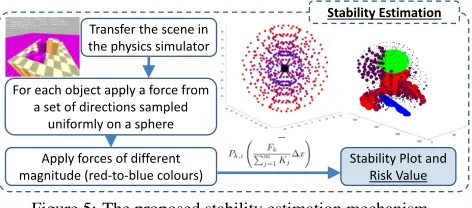
Transfer the scene in the physics simulator
For each object apply a force from a set of directions sampled
uniformly on a sphere
Apply forces of different
magnitude (red-to-blue colours) Stability Plot and Risk Value
Stability Estimation
Figure 5: The proposed stability estimation mechanism.
Other risk elements obtained from related acquisition de-vices, such as thermal cameras, material analysis etc can also be utilised and their impact added to the risk score. This ensures the proposed framework is extendable as re-quired.
For the purpose of this paper we define the cumulative risk scoreRas a function of the weighted elements, stability Sand hazard featuresH.
R=f(wSS, wHH) (2)
3.3. Proposed Stability Estimation Mechanism
The proposed novel methodology for scene stability es-timation is based on Newtonian physics. To evaluate sta-bility, forces are applied to objects within the scene and the resultant outputs measured (Figure5). Statistical analysis on those outputs can be performed providing information about the properties of the scene. Consequently, allowing us to model the behavior of segmented objects and compute the energy output from the applied forces.
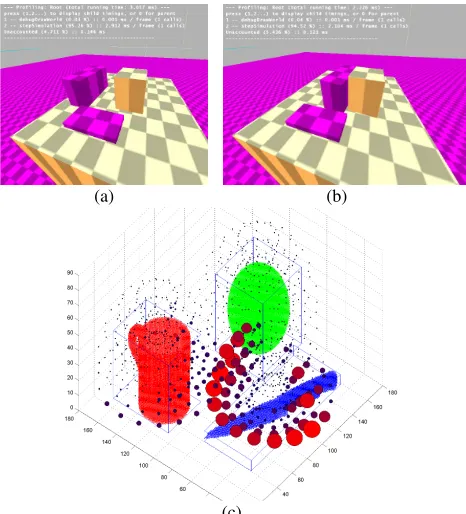
[image:3.612.311.547.73.177.2](a) (b)
[image:4.612.58.291.70.327.2](c)
Figure 6: Stability evaluation process using Newtonian Physics (a) Initial layout in the physics simulation (b) Collision occurring during the simulation and (c) Stability Plot with the circles around the objects indicating the direction of instability and the radius corresponding to the severity.
Stabilitysfor a forcekon a given objectiis considered as a dimensionless quantity and is defined as the ratio of the applied forceFkover the summed kinetic energyKjfor all
the objectsmin the scene. This is scaled by the probability Pk,iof the force being applied.
sk,i =Pk,i
Fk
Pm
j=1Kj
∆x !
(3)
whereKj =P
T
t=1
1 2M Vt
2
represents the accumulated ki-netic energy of the objectjover timeT from a simulation obtained using numerical integration. HereM represents mass and V the velocity of the objectj at a given timet.
∆xis the object’s displacement, but since the kinetic en-ergy is calculated numerically over fixed length intervals, this value is equal to one.
ProbabilityPk,irepresents the likelihood of a given force
Fk being applied to objecti. This is defined as whether
the force could collide with the object without hitting first another entity within the scene. For example forces from below an object on a plane would collide with the surface first therefore would not be considered.
ForcesF of different strengths are applied to the cen-ter of each bounding box (object) during the simulation, with directions sampled from a uniform distribution of an-gles over a sphere. The resultant overall kinetic energyK for each objectjis calculated. By analysing the amount of
For all the voxelized objects in the
scenes of 3DRS apply 3DVoxel HOG using Adaboost Train a model
Hazard Features Estimation 3D Voxel HOG Descriptor
Manually select the sharp features
For each upcoming voxelized object
in a new scene apply 3DVoxel HOG Test using the above model Obtain the Risk Value
Figure 7: The proposed hazard classification system.
kinetic energy produced by each object for each force we can ascertain if, during the course of that simulation, an ob-ject has been dislodged from the surface or if other obob-jects within a scene have been affected. By varying the strength of force we build up a picture of how unstable an object is in its environment. The total stabilitySof a scene is given as the sum of the estimated stabilitysfor each forcekapplied to each objectj.
S=
r
X
k=1
m
X
j=1
sk,j (4)
The outcome of this process will allow us to differenti-ate between the case of an object (e.g. glass bottle) being placed at the center of a table or at the edge, evaluating with enough precision the stability of each scene, (Figure6).
3.4. Novel Hazard Feature Descriptor
The application of three dimensional descriptors to iden-tify the properties of an object is a new concept. In the proposed framework rather than focusing on object recogni-tion, the detection of hazard features is the core vision prob-lem. This introduces the novel classification task of recog-nising hazardous areas in a scene. The novel 3D Voxel HOG descriptor is introduced, which is specifically designed to be suitable for local feature recognition whilst also considering an objects’ density. An overview of the proposed approach is shown in Figure7.
The traditional HOG uses the normalized combination of gradient vectors from a given number of pixels to build up a histogram of binned angles that relate to the feature. We extend this process to the third dimension though the use of voxels and 2D histograms. The process begins by breaking the voxel volume up into set features spacesf comprised of a number of cubic 3D cellsc, which in turn is made up of voxels v. For each voxel within a cell the filter mask
[−1,0,1]is applied to its neighbouring voxels in all three dimensions giving us the gradient vector~g.
[image:4.612.307.549.73.188.2](a) (b)
5 10 15 2
4 6
8 0
0.1 0.2 0.3 0.4
Surf for Block1 Feature1
(c)
0 20 40 60 80 100 120 140 160 180 0
0.05 0.1 0.15 0.2 0.25
[image:5.612.59.277.70.242.2](d)
Figure 8: 3D Voxel HOG feature from a cube wall test case, (a) visualised on its object in 3D, (b) the same 3D representation in two different orientations, (c) as a 2D Histogram and (d) as a 162 dimension feature vector
zenithφangles.
(θ, φ) = (cos−1(q gz
g2
x+g2y+gz2
),tan−1(gy, gx)) (5)
Additionally a weightwis defined for each voxel, which is used to scale its contribution to its cell’s 2D histogram. This is given by the mean value of the voxels within a given three dimensional kernel indicating the density over this area. By applying this weight, the proposed approach provides accu-rate estimates even in the presence of noise.
Once these values are established the voxels within each cell are binned into a 2D histogramhaccording to theirθ andφangles. The value added to the specified bin is given as the weighted magnitude of the vectorwk~gk. Finally all the histograms for each cell within a feature hf are
nor-malised using theL2norm.
hf →
hf
p
k~gk2 2+e2
(6)
The obtained features are then vectorised and used by the learning mechanism to create a classification model.
~
x3DV HOG={h1,1, ..., h1,ϕ, ..., hθ,ϕ} (7)
The resultant 2D histograms can be visualised, and present a way of identifying different types of features within an object (Figure 8c). Another form of visualisa-tion plots each possible gradient vector within local 3D histograms, showing the most common gradient vectors as stronger (see figure8a,b).
Training is then carried out to create a model to classify safe and unsafe local features. The defined features of an unknown object can then be tested against this model and return a binary classification for each feature as either haz-ardous or not. This data then forms the hazard component of the Risk score.
3D HOG Proposed 3D VHOG Given 3D Objects
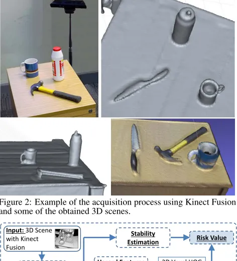
Figure 9: Example showing the differences of the proposed 3D Voxel HOG features with the 3D HOG [27] indicating that the ob-jects’ internal density affects the proposed 3D VHOG descriptor.
One of the primary advantages of the proposed 3D Voxel HOG (3D VHOG) is the consideration of not only the faces of a mesh but also the area within as well. This ensures that no additional artifacts are created within the data that may lead to false classifications, additionally the density of an object is also taken into consideration (e.g. empty and full cup). This allows transference of the methodology to other areas such as medical imaging, for example the proposed method could detect defects such as osteoporosis in bone MRI scans which existing methods would not. A visual comparison of the 3D HOG features suggested in [3,27] against 3D VHOG is shown in figure9 indicating that the proposed method does not introduce erroneous information in the internal areas of an object. Importantly 3D VHOG returns one 2D histogram (visualised in 3D) per cell (Figure
8), as apposed to the other methods that provide multiple 1D histograms (visualised in 2D).
The use of voxel weighting smooths the edges of an ob-ject cluster ensuring robustness against noisy input data. Due to the local nature of the proposed feature, issues re-lated to the normalization of a mesh are avoided, removing a potentially complex pre-processing step.
The pseudo code for the 3D Voxel HOG implementation is outlined below.
1. choose Size of Cell and Block 2. FOREACH Voxel v DO
3. compute Weight w, Gradient (θ, φ), Vector Magnitude k~gk
4. FOREACH Cell c in Feature f DO
5. create blockHist(theta_bins, phi_bins) 6. FOREACH voxel v in c DO
7. insert wk~gk into blockHist (θ, φ) 8. L2Normalize(blockHist in Feature)
[image:5.612.311.544.73.183.2]clas-sifiers with the lowest error margin are used to define the next in a ‘greedy fashion’. Regarding the proposed features in both cases givenN training examples(~x1, ..., ~xN), the
corresponding labels(y1, ..., yN)withyi ∈ {−1,1}, and
an initial distribution of weightsW1(i)a strong classifica-tion modelH(x)is obtained based on the weak classifiersh. The weak classifiers are trained over a number of iterations Qusing the weights’ distributionWt. In each iteration the
errortis estimated based on the current weightsWt, that
are updated before the next iteration.
Wt+1(i) =Wt(i) exp(−atyiht(xi))/Zt (8)
whereat =−12log(t/(1−t))andZt = 2
p
t(1−t)
is a normalization factor. The strong classifier is defined as
H(x) =sign(r(x)), wherer(x) =~ak·~~ha(kx)
1 .
Regarding the boosting approach, because of the way weak classifiers are selected a complicated feature problem can be broken down and classified using a sparse classi-fication rule, based on only a few features. This makes computation much faster as only a subset of the features are used. This is essential if the methodology is to be im-plemented in a real time scenario. Another advantage of this approach is the explicit minimisation of error, whilst implicitly maximising the margin. This ensures the final strong classifier is general avoiding the problems of over-fitting. Another similar boosting technique uses Support Vector Machines(SVM). This also provides a non linear, ro-bust classifier, however tends to have higher computational requirements. This is due to their classifier taking into ac-count all the features in a vector as apposed to a subset [23]. Finally, in order to define a second elementEof the risk scoreRin equation (1) related to the ‘hazard features’ the obtained outcomes from the classification process above are utilised.
H3DV HOG= 1
m
m
X
j=1
PM
k=1wHG(j, k)
PM
k=1G(j, k)
!
Hω= 1
m
m
X
j=1
wD(j) (9)
wherewD=f(x)normalised andG= 12(sign(f(x))+1).
4. Results
4.1. Experiment Environment
In our experiments, scenes containing mainly household objects and toys placed on a surface were utilised. In order to obtain a ground truth for each scene and to ensure that the parameters of the tests are fully controllable and repeat-able the objects were manually placed in specific locations on the given surface. To effectively test this problem and as
[image:6.612.315.540.72.139.2](a) (b) (c)
Figure 10: An example scenario with each of its iterations. The level of complexity is increased from a simple layout(a) to a com-plex (c).
no existing dataset fits the proposed work, a new dataset for risk estimation in 3D scenes (3DRS) was created compris-ing of36scenes captured using RGBD cameras. These36
scenes are split into12different scenarios, each containing
3 objects. Each of these has3stability levels in terms of scene complexity, i.e. the objects are moved closer together on the plain (Figure10). These include examples of ‘haz-ardous’ (scissors, stanley (open), screwdriver, plane, pencil, pen knife (open), knife, fountain pen, fork, cleaver, ball-point pen, axe) and safe (vase, stanley (closed), spoon, rubix cube, pen knife (closed), mug, mouse, laptop, lamp, frame, bowl, bottle, ball) objects, with multiple instances for most of them. Additionally an object’s material is not defined in this work, as such objects within a scene specified as being made from the same material and have the same friction (1) and angular dampening coefficients (0.4). The 3D recon-structed models were processed to remove some noise but also to close any gaps in the mesh since this is essential for the voxelization stage. Regarding the voxelization process of the 3DRS dataset, a set resolution of 256 cubic voxels was defined for the voxel volume. The resolution has a di-rect impact on computation time for each stage and as such this represents a reasonable trade off for processing time against object detail. For segmentation the the Mean Shift algorithm was found to be the most efficient at separating the objects across all the complexity levels.
4.2. Scene Stability
(a)
(b)
(c)
1 2 3
500 550 600 650
Stability Level
Energy
Example Scene Stability Test
[image:7.612.75.269.68.431.2](d)
Figure 11: Results visualised using spheres placed around the ob-ject indicating the direction and the level of instability in case (a) Far Left Corner, (b) Left Side and (c) Centered and (d) Scene en-ergy per stability level in graph form.
uniform sampled points along a sphere and the scenes’ over-all stability quantified according to equations (3), (4). Some stability visualizations are presented in Figure12. The re-sultant graph demonstrates that as the objects get closer to-gether and positioned more centrally the scenes risk is re-duced (Figure13). Due to the nature of this type of evalu-ation, a ground truth is unnecessary as we are quantifying or estimating an attribute of a scene. This allows for good generalisation to other scene scenarios as the technique re-lies on the measurement of a physics simulation rather than a supervised classification technique.
4.3. 3D Voxel HOG Experiments
The second component proposed to evaluate the risk level of a scene relates to an objects’ properties or in this case it’s ‘hazardous features’. The evaluation of risk or what constitutes a hazard is contextual and as such varies in each situation. One of the areas this work aims to expand is the implementation of smart homes and domestic robotics. As
0 50
100 150
2000 50
100 150
200 0
20 40 60
0
50
100
150
20050
100 150
200 0
[image:7.612.311.544.71.283.2]20 40 60 80 100
Figure 12: Scenes with the risk and stability levels visualised.
Stability Level
1 2 3
Instability Value
0 0.05 0.1 0.15 0.2 0.25 0.3 0.35
Instability Values for each scenario per Stability Level (Proposed Method)
Stability Level
1 2 3
Instability Value
0 0.05 0.1 0.15 0.2 0.25 0.3
0.35Instability Values for each scenario per Stability Level (Zheng et al.)
Figure 13: Stability Value for each scenario per Stability Level, (a) Proposed methods, (b) Work presented in [37]. The vertical axis indicates the stability value obtained using equation (4), and the horizontal axis indicates the four different stability levels shown in figure10. Each of the lines corresponds to one of the scenes. Higher the stability value less stable is the scene.
these technologies are often utilised in environments where people reside, our definition of risk relates to the household environment. However these environments also suffer from variance, for example a smart enabled household with chil-dren would consider many more things hazardous than one without. In this case we look to define all structures of the objects in the 3DRS dataset with sharp edges and corners.
Figure 14: The 3D Voxel HOG visualisation of objects with the classified areas as hazardous coloured red.
Feature F1 Sensitivity Accuracy
3D HOG [27] 0.533 0.500 0.363
3D Sift [28] 0.333 0.250 0.272
3D Harris [30] 0.200 0.110 0.272
[image:8.612.58.276.72.208.2]3D VHOG 0.625 0.625 0.454
Table 1: Feature comparison against other existing 3D descriptors.
Object B C F H K M
Hazard Score 0 0.5 0.5 0.6 0.5 0
Object P Pl S Sd Bt
Hazard Score 0.7 0.6 0.3 0.6 0
Table 2: Hazard scores for the testing objects with higher val-ues indicating higher risk (e.g. presence of hazardous features). Some of the objects are listed below: Ball, Cleaver, Fork, Hammer, Knife, Mug, Pencil, Plane, Scissors, Screwdriver, Bottle. Values obtained using Equation (9).
classified almost all features as hazardous, highlighting it as ineffective for use in the local space. In Figure14 exam-ples of the 3D VHOG features for some of the objects are shown.
Since the ‘hazard features’ of the testing objects have been estimated based on the proposed 3D VHOG descrip-tor and the classification mechanism, the level of risk based on the objects’ characteristics is defined using the equation (9). The obtained results for some of the testing objects are shown in Table2indicating that the proposed method pro-vides reasonable and accurate estimates.
4.4. Overall scene risk evaluation
An overall confidence (risk) score for each scene is fi-nally estimated combining the previous partial results using equation (1). All the results are shown in table3.
5. Conclusions
In this work the concept of risk analysis is considered for 3D scenes. A novel approach to evaluating scene stability
Scenario 1 2 3 4 5
Risk 0.8 0.5 0.6 0.5 0.6
Scenario 6 7 8 9 10
Risk 0.6 0.7 0 0.7 0.8
Table 3: The overall risk value for each one of the scenes. Values obtained using Equation (1) (4) (9).
is given using Newtonian Physics. The 3D Voxel HOG de-scriptor is introduced and designed to represent the intrinsic properties of an object. When compared with other state of the art features, 3D VHOG provided the highest accuracy in risk detection. Additionally 3D VHOG has the advantages of considering an object’s density as well avoiding issues relating to the normalization of a mesh. Furthermore, a new dataset was developed for 3D scene risk analysis and exper-iments were performed showing that the proposed frame-work has the potential to accurately measure risks in scenes.
References
[1] P. W. Battaglia, J. B. Hamrick, and J. B. Tenenbaum. Sim-ulation as an engine of physical scene understanding. Pro-ceedings of the National Academy of Sciences of the United States of America, 110(45):18327–32, Nov. 2013.2
[2] A. N. Belbachir, A. Nowakowska, S. Schraml, G. Wiesmann, and R. Sablatnig. Event-driven feature analysis in a 4D spa-tiotemporal representation for ambient assisted living. 2011 IEEE International Conference on Computer Vision Work-shops (ICCV WorkWork-shops), pages 1570–1577, Nov. 2011.2
[3] N. Buch, M. Cracknell, J. Orwell, and S. A. Velastin. Vehicle localisation and classification in urban CCTV streams.Proc. 16th ITS WC, pages 1–8, 2009.2,5
[4] N. Buch, S. A. Velastin, and J. Orwell. A Review of Com-puter Vision Techniques for the Analysis of Urban Traffic.
IEEE Transactions on Intelligent Transportation Systems, 12(3):920–939, Sept. 2011.1
[5] L. Chen, C. D. Nugent, and H. Wang. A
Knowledge-Driven Approach to Activity Recognition in Smart Homes.
IEEE TRANSACTIONS ON KNOWLEDGE AND DATA EN-GINEERING, 24(6):961–974, 2012.1
[6] N. Dalal and B. Triggs. Histograms of oriented gradients for human detection. InProceedings - 2005 IEEE Computer Society Conference on Computer Vision and Pattern Recog-nition, CVPR 2005, volume I, pages 886–893, 2005.2
[7] C. Do and B. Javidi. 3D integral imaging reconstruction of occluded objects using independent component analysis-based K-means clustering. Display Technology, Journal of, 6(7):257–262, 2010.3
[8] R. Dupre, V. Argyriou, G. Tzimiropoulos, and D. Greenhill. 3D Voxel HOG and Risk Estimation. InIEEE DSP Singa-pore, 2015.2
[9] D. Engel and C. Curio. Towards robust scene analysis: A ver-satile mid-level feature framework. kyb.tuebingen.mpg.de, page 2009, 2009.2
[image:8.612.60.274.234.298.2]Recognition, 2009. CVPR 2009. IEEE Conference on, pages 1778–1785. IEEE, 2009.2
[11] A. Fossati, H. Grabner, and L. Van Gool. Exploiting Phys-ical Inconsistencies for 3D Scene Understanding. In 3D Imaging, Modeling, Processing, Visualization and Transmis-sion (3DIMPVT), 2012 Second International Conference on, pages 136–143. IEEE, 2012.2
[12] Y. Freund and R. Schapire. A desicion-theoretic generaliza-tion of on-line learning and an applicageneraliza-tion to boosting. Com-putational learning theory, 1995.1
[13] A. Godil and A. Wagan. Salient local 3D features for 3D shape retrieval. IS&T/SPIE Electronic Imaging, (Shrec), 2011.2
[14] S. Izadi, A. Davison, A. Fitzgibbon, D. Kim, O. Hilliges, D. Molyneaux, R. Newcombe, P. Kohli, J. Shotton, S. Hodges, and D. Freeman. Kinect Fusion: Real-time 3D Reconstruction and Interaction Using a Moving Depth Cam-era. In Proceedings of the 24th annual ACM symposium on User interface software and technology - UIST ’11, page 559, 2011.3
[15] Z. Jia, A. Gallagher, A. Saxena, and T. Chen. 3D-Based Rea-soning with Blocks, Support, and Stability.2013 IEEE Con-ference on Computer Vision and Pattern Recognition, pages 1–8, June 2013.2
[16] A. Kl¨aser, M. Marszaek, C. Schmid, and A. Zisserman. Hu-man focused action localization in video. InTrends and Top-ics in Computer Vision, volume 6553 LNCS, pages 219–233, 2012.2
[17] Y. Kobayashi, T. Morimoto, I. Sato, Y. Mukaigawa, and K. Ikeuchi. BRDF Estimation of Structural Color Object by Using Hyper Spectral Image. InComputer Vision Workshops (ICCVW), 2013 IEEE International Conference on, pages 915–922, Dec. 2013.3
[18] R. Koch. Dynamic 3-D scene analysis through synthesis feedback control.Pattern Analysis and Machine Intelligence, IEEE Transactions on, 15(6):556–568, 1993.2
[19] S. J. Koppal and S. G. Narasimhan. Clustering appearance for scene analysis. InComputer Vision and Pattern Recogni-tion, 2006 IEEE Computer Society Conference on, volume 2, pages 1323–1330. IEEE, 2006.2
[20] S. J. Koppal and S. G. Narasimhan. Appearance derivatives for isonormal clustering of scenes.Pattern Analysis and Ma-chine Intelligence, IEEE Transactions on, 31(8):1375–1385, 2009.2
[21] D. Lee, M. Hebert, and T. Kanade. Geometric reasoning for single image structure recovery. 2009 IEEE Conference on Computer Vision and Pattern Recognition, pages 2136– 2143, June 2009.2
[22] B. Leibe, N. Cornelis, K. Cornelis, and L. Van Gool. Dy-namic 3D Scene Analysis from a Moving Vehicle. 2007 IEEE Conference on Computer Vision and Pattern Recog-nition, pages 1–8, June 2007.2
[23] J. H. Morra, Z. Tu, L. G. Apostolova, A. E. Green, A. W. Toga, and P. M. Thompson. Comparison of AdaBoost and support vector machines for detecting Alzheimer’s disease through automated hippocampal segmentation. IEEE trans-actions on medical imaging, 29(1):30–43, Jan. 2010.6
[24] K. Onishi, T. Takiguchi, and Y. Ariki. 3D human posture estimation using the HOG features from monocular image.
2008 19th International Conference on Pattern Recognition, pages 3–6, 2008.2
[25] A. Prest, V. Ferrari, and C. Schmid. Explicit model-ing of human-object interactions in realistic videos. IEEE transactions on pattern analysis and machine intelligence, 35(4):835–48, Apr. 2013.2
[26] Real-Time Physics Simulation. Bullet User Manual and API Documentation, 2012.6
[27] M. Scherer, M. Walter, and T. Schreck. Histograms of ori-ented gradients for 3d object retrieval. Proceedings of the WSCG, 2010.2,5,8
[28] P. Scovanner, S. Ali, and M. Shah. A 3-dimensional sift de-scriptor and its application to action recognition. Proceedings of the 15th international conference on Multimedia -MULTIMEDIA ’07, (c):357, 2007.2,8
[29] J. Shotton, A. Fitzgibbon, M. Cook, T. Sharp, M. Finocchio, R. Moore, A. Kipman, and A. Blake. Real-time human pose recognition in parts from single depth images. Cvpr 2011, pages 1297–1304, June 2011.2
[30] I. Sipiran and B. Bustos. Harris 3D: a robust extension of the Harris operator for interest point detection on 3D meshes.
The Visual Computer, 27(11):963–976, July 2011.2,8
[31] E. Stone and M. Skubic. Evaluation of an Inexpensive Depth Camera for Passive In-Home Fall Risk Assessment. Pro-ceedings of the 5th International ICST Conference on Perva-sive Computing Technologies for Healthcare, 2011.2
[32] A. Swadzba, N. Beuter, S. Wachsmuth, and F. Kummert. Dynamic 3D scene analysis for acquiring articulated scene models. 2010 IEEE International Conference on Robotics and Automation, pages 134–141, May 2010.1
[33] S. Tang, X. Wang, X. Lv, T. X. Han, J. Keller, Z. He, M. Sku-bic, and S. Lao. Histogram of oriented normal vectors for object recognition with a depth sensor. InComputer Vision-ACCV, volume 7725 LNCS, pages 525–538, 2013.2
[34] A. Trevor, S. Gedikli, R. B. Rusu, and H. I. Christensen. Ef-ficient organized point cloud segmentation with connected components. InProceedings of Semantic Perception Map-ping and Exploration, pages 1–6, 2013.3
[35] J. Wang, C. Zhang, W. Zhu, Z. Zhang, Z. Xiong, and P. A. Chou. 3D scene reconstruction by multiple structured-light based commodity depth cameras. InICASSP, IEEE Interna-tional Conference on Acoustics, Speech and Signal Process-ing - ProceedProcess-ings, pages 5429–5432, 2012.3
[36] O. Wang, P. Gunawardane, S. Scher, and J. Davis. Material classification using BRDF slices. InComputer Vision and Pattern Recognition, 2009. CVPR 2009. IEEE Conference on, pages 2805–2811, June 2009.3
[37] B. Zheng, Y. Zhao, and J. Yu. Detecting Potential Falling Ob-jects by Inferring Human Action and Natural Disturbance.
IEEE Int. Conf. on Robotics, 2014.2,7
[38] B. Zheng, Y. Zhao, J. C. Yu, K. Ikeuchi, and S.-C. Zhu. Be-yond Point Clouds: Scene Understanding by Reasoning Ge-ometry and Physics.2013 IEEE Conference on Computer Vi-sion and Pattern Recognition, pages 3127–3134, June 2013.
![Figure 9: Example showing the differences of the proposed 3DVoxel HOG features with the 3D HOG [27] indicating that the ob-jects’ internal density affects the proposed 3D VHOG descriptor.](https://thumb-us.123doks.com/thumbv2/123dok_us/8668788.376481/5.612.59.277.70.242/example-differences-proposed-features-indicating-internal-proposed-descriptor.webp)