Response Properties and Adaptation of Neurones Sensitive to Image Motion in the Butterfly Papilio Aegeus

Printed in Great Britain © The Company of Biologists Limited 1991

RESPONSE PROPERTIES AND ADAPTATION OF NEURONES

SENSITIVE TO IMAGE MOTION IN THE BUTTERFLY

PAPILIO AEGEUS

BY T. MADDESS, R. A. DUBOIS AND M. R. IBBOTSON

Centre for Visual Sciences, Research School of Biological Sciences, PO Box 475, Canberra, ACT 2601, Australia

Accepted 8 July 1991

Summary

Wide-field direction-selective neurones from the optic lobes of the butterfly

Papilio aegeus show some properties similar to those displayed by the large

neurones of the fly lobula plate. Temporal and spatial frequency threshold tuning curves show that butterfly optic lobe neurones sensitive to different directions of image motion are fed by presynaptic subunits similar to those of the fly. However, unlike fly lobula plate neurones, the butterfly optic lobe neurones show a steep low-spatial-frequency roll-off which persists even at high temporal frequencies. Also exceptional is the temporal resolution of rapid changes in image speed by the butterfly neurones. When the cells are adapted to continuous motion their responses indicate a further increase in temporal resolution. Evidence is provided that in any one state of adaptation the neurones may be thought of as piece-wise linear and, thus, their responses can be predicted by convolution with a velocity kernel measured for that adaptation state. Adaptation to continuous motion results in the cells responding to motion in proportion to the mean motion signal. Motion in the non-preferred direction also appears to adapt the cells. Velocity impulse responses of both butterfly and blowfly neurones were determined with one-dimensional gratings and two-dimensional textured patterns and the results for the two stimuli are shown to be very similar.

Introduction

Motion-sensitive neurones in Lepidoptera have been known for some time (Collett and Blest, 1966), the majority of work having been on hawk moths (Collett, 1970, 1971, 1972; Rind, 1983a,b) although there are reports of such cells in butterflies (e.g. Swihart, 1969). The temporal and spatial frequency tuning of motion-sensitive interneurones of blowflies has been investigated at contrast threshold to quantify their responses and to gain some insight into their presynaptic circuitry (e.g. Zaagman et al. 1978; Dvorak et al. 1980; Mastebroek et

al. 1980; Srinivasan and Dvorak, 1980). We take the same approach here to

determine the characteristics of subunits presynaptic to a class of motion-sensitive neurones connecting the medulla and midbrain of butterflies. We have provided detailed information about the anatomy and directional selectivity of these cells elsewhere (Ibbotson et al. 1991).

In addition to an examination of the spatial and temporal tuning of the large medulla neurones, we also examine the cells' adaptation to image motion by examining their velocity impulse responses in a variety of adapting conditions. Srinivasan (1983) and Zaagman et al. (1983) were the first to characterize motion-sensitive neurones by their motion or velocity impulse responses. The velocity impulse response is simply the response to a brief displacement of the image. If the neurone's response to the stimulus is linear then the response to any complex motion stimulus can be predicted by convolution of the time-varying velocity signal with a scaled version of the impulse response, which we refer to here as the velocity 'kernel'. Further explanation of the meaning of the velocity kernels is provided in the Materials and methods and Discussion sections.

Investigation of the HI neurone in the fly (Zaagman et al. 1983) showed that the width of the impulse response, and thus also the integration time, was not constant but instead depended upon the time-averaged rate of stimulation. At high stimulation rates the impulse response narrows and the integration time can drop to about 10ms. With very low stimulation rates ( > l H z ) the integration time expands to about 300 ms (Zaagman et al. 1983; Maddess, 1986). This is a significant departure from linearity in the neurones' response to image velocity. Neverthe-less, it is possible that the neurones may be thought of as being piece-wise linear, i.e. linear within any one adaptation state, in which case the velocity kernel may still characterise a neurone's response in a given adaptation state. The experiments that follow examine two questions. First, the extent to which the medulla neurones of Papilio aegeus change their response characteristics as a function of adaptation to different velocities. Second, whether the cells can be thought of as being piece-wise linear, i.e. whether the impulse response obtained in a given state of adaptation is useful for characterising the neurone's response in that adaptation state. Two further sets of experiments examine whether the neurones adhere to Weber's law with changes in adaptation state. Some experiments using two-dimensional textured stimuli are compared to the results obtained for one-dimensional gratings.

173

correlates of the adaptation of motion-sensitive neurones have also been reported for the fly (Kirschfeld, 1989).

Materials and methods Animals and preparation

Butterflies, Papilio aegeus aegeus Don., were collected locally or raised from caterpillars found in the Canberra area. Male and female butterflies were used, and no sex-specific response characteristics were observed. After their wings had been clipped, the animals were waxed (50% beeswax and 50% cello resin) to an articulated stand. The head was tilted slightly forward, the scales of the neck region removed and a hole was cut to reveal the lobula region of the right optic lobe. The large tracheae covering the optic lobe were left largely intact and tungsten in glass electrodes (Merrill and Ainsworth, 1972) were guided between the tracheae to reach the brain. A landmark used in the positioning of the electrodes was a pigmented blob that is always found on the dorsal surface of the optic lobe. Subsequent anatomical investigations of Papilio aegeus have revealed that this pigmented blob lies over the posterior optic tract (Fig. 1), which contains the axons of the large medulla neurones: 55 intracellular fills of cells in this region

100 ^m

yielded only neurones of this class (Ibbotson etal. 1991). It is, therefore, expected that the bulk of the recordings presented here are from the large medulla neurones. For comparison with previous studies, we also examined the responses of lobula plate neurones in the blowfly Lucilia cuprina dorsalus R.-D. Standard recording techniques were used for the flies (Maddess and Laughlin, 1985). The data presented are based on records from 29 butterfly and 5 blowfly neurones on which experiments were completed and several more records from incomplete experiments.

Since temperature can affect the dynamics of the phototransduction process in the insect retina (Payne and Howard, 1981), all comparative fly/butterfly experiments were carried out in a temperature-controlled laboratory, the tem-perature variation of the room being 23±2°C. All animals were prepared for the experiment in this same room and the preparation period allowed the room to come to equilibrium temperature. Room temperature was continuously measured by a recording thermometer placed about 70 cm from the animal in the Faraday cage of the recording set-up. Experiments where butterfly neurones were not compared with flies were conducted in another room where the temperature ranged from 26 to 28 °C (see Howard et al. 1984).

Records from single units were amplified by standard methods and converted to uniform 0.5 ms pulses after detection by a level discriminator. Pulses were either recorded by the computer controlling the stimulus (Digital Electronics Company LSI-11/03 or NEC 386/20) and/or tape recorded for later, off-line analysis. It was difficult to orient the animals exactly to the cathode-ray tube (CRT) face because their black eyes obscure their pseudopupils, but an attempt was made to have the animals squarely view the centre of the CRT. Comparisons of receptive field profiles from ipsilaterally and contralaterally recorded cells showed that horizontal alignment was good to within ±5°. In this paper ipsilateral is taken to mean that the cell's excitatory receptive field was primarily on the same side of the head as the recording electrode. The relatively flat receptive fields of vertical cells made accuracy of alignment in the vertical direction less certain.

Experiments and stimuli

The preferred directions of a cell were assessed using sinusoidal gratings at a variety of orientations. Directional selectivity was assessed in trials where the grating was moved for 3 s periods of to-and-fro motion between equal periods when the grating remained stationary on the CRT. When the preferred orientation had been established, a cell's receptive field was determined by repeatedly sweeping a bright (180% of the mean luminance) bar (1.2° wide at the CRT centre) across the CRT.

threshold was determined by comparison of the mean spike counts obtained from the periods when the stimulus moved and when it was stationary. Mean spike counts were determined for 8-10 repetitions. A stimulus was taken to be at threshold when the mean spike number obtained from the moving phase minus one standard deviation was just less than the mean count from the stationary phase plus one standard deviation. At first the threshold temporal tuning was established with the same grating used to find the preferred orientation. Once the optimum temporal frequency had been established, contrast thresholds were determined for different spatial frequencies. The stimulus generating equipment has been previously described (Maddess and Laughlin, 1985) and the mean luminance for all the experiments described so far was 4cdm~2.

Velocity impulse responses were determined in a different stimulus arrange-ment. Sinusoidal gratings of 0.2 cycles degree"1 were presented in a rectangular window of 50°x60° using an HP1332A monitor at a mean luminance of 40cdm~2 (green P31 phosphor) and with a video frame refresh period of 5.35 ms. These experiments involved measuring the neurones' responses to brief impulses of velocity presented against a steady adapting velocity. The effects of afterimages (Maddess, 1986) were minimised by varying the spatial phase of the grating at which the velocity impulse occurred in each trial. Afterimage effects were thus averaged out.

In these experiments the inter-spike interval was recorded with a resolution of 0.01ms. These data were reorganised into histograms with lms bin widths. The 1 ms bins allowed accurate measurement of response delays but at the same time meant that the histograms contained information at frequencies up to 500 Hz. It was clear, however, from examination of these raw histograms that the infor-mation of interest was at lower frequencies and this was obscured by high-frequency noise. Therefore, simultaneously to remove the high-high-frequency noise and to preserve information about response delay, these histograms were digitally filtered using a recursive zero-phase shift algorithm with a high-frequency cut-off of 100, 200 or 250 Hz depending on the frequency band of interest. The zero-phase shift process ensured that, while high-frequency noise was removed from the traces, the 'delay' of the lower-frequency components of interest was unchanged.

A set of four separate tests was repeated several times on each of the nine neurones studied in the velocity impulse experiments. The four experiments examined (1) the response of the neurone to impulsive jumps of the image against various adapting background velocities, (2) the ability of the cell to resolve two closely paired impulsive jumps, (3) the ability of the cells to resolve the time courses of different jumps which had the same total displacement and (4) the possibility that the cells on adapting show a gain control that follows Weber's law. Trials from these four experiments were interleaved and then repeated for about 6h to obtain sufficient data from each cell.

these tests provided controls to confirm that the responses generated by textured stimuli were consistent with previous results obtained for one-dimensional grating stimuli (Srinivasan, 1983; Maddess and Laughlin, 1985). Experiments of this kind were completed for 10 cells. The background luminance was provided by dim incandescent room lights and was 100 times dimmer than the dots. Computer simulation models of the blurring effects of the flies' optics on this stimulus indicate that the stimulus presented an average contrast of about 100 % to the photoreceptors. The coordinates of the dots were obtained from a table of random numbers with an even distribution. The matrix of dots spanned the CRT along its horizontal axis (63°). The minimum distance between the dots was 1.3° (at the CRT centre). The dots were redrawn every 6.57ms. The smallest dot displace-ment allowed positional incredisplace-ments of 0.13° which, in conjunction with the refresh time of 6.57 ms, allowed drift rates as slow as 1.98 degrees s"1. The trial time for all these experiments was 1.68 s, or 256 refreshed 'frames' of dots, and between 100 and 400 trials were averaged for each test condition. Velocity increments or decrements were presented on top of an adapting velocity which varied from 0 to 80 degrees s"1.

Background to velocity kernels

The Fourier transform of the velocity kernel yields the amplitude spectrum of the system. The Fourier transform of the autocorrelation function of the kernel is the power spectrum. Thus, the impulse response potentially provides a quicker method for obtaining the same information as harmonic analysis. So, rather than laboriously testing the response of a neurone with a range of frequencies, the same information can be obtained simply by measuring the response to a brief stimulus. In the case of the velocity impulse response or kernel, the frequency domain representation describes responses to frequencies of back-and-forth oscillations of the image, not the contrast frequency.

that the 'equivalent width' of the autocorrelation function of the impulse response is exactly equal to the reciprocal of the equivalent width of the power spectrum:

autocorrelation(/)df ,„.

_ power spectrum(O) . .

autocorrelation(O) f°° /T^JT-'

power spectrum(F)dF

J —OO

where t is time and F is frequency.

Results

Receptive fields and general response characteristics

Receptive fields of the neurones were characterised by moving thin bars across the face of the CRT (see Materials and methods) at a variety of drift velocities. The receptive field of an ipsilaterally recorded cell sensitive to downward motion (Fig. 2) shows several characteristics typical of the vertical cells, six of which had their receptive fields determined in detail. The receptive field sensitivity profiles of vertical cells were rather flat: only by removing a d.c. bias of 60 impulses s"1 can a slight preference for stimuli in the ventral visual field be seen for the cell of Fig. 2A. The receptive field (Fig. 2C) and orientation preference (Fig. 2D) of a contralaterally recorded horizontal cell from the animal's right optic lobe show marked similarity to the behaviour of the fly neurone HI. However, 55 intracellular dye injections (Ibbotson et al. 1991) at the same site (Fig. 1) failed to reveal any lobula plate neurones, so it appears that this cell may be a bilateral medulla neurone like that described by Milde (1988) in the moth Manduca sexta.

When assessing cells' directional preferences, some trials of 60s duration were conducted to reveal any adaptive effects similar to those reported for fly lobula plate neurones (Maddess and Laughlin, 1985). In the two examples shown (Fig. 2B,D) there is a conspicuous change in sensitivity suggested by the gradually waning response during the 15 s of preferred motion. Notice that the cells' responses do not come to a steady state even over a period of 15 s. Also notable is the fact that the stimulus contrast in both cases was only 0.4, which is not saturating and, therefore, the adaptation is proceeding without the stimulus driving the cell very hard. The temporal frequencies used to produce the responses shown in Fig. 2B,D were the moderately high rates of 6 and 8 Hz, respectively, and so, given that the contrasts were not saturating, the likely source of response decline is temporal-frequency-dependent adaptation (Maddess and Laughlin, 1985).

Cell PD4 Cell PD4

- 4 0 - 2 0

Cell PR1

40

3 20

0

-- 2 0

Cell PR1 D

"•Hi

20 40 60

100 80 60 40 20 0 - 4 0

E

-P1R2

1 1

(--) and

A

P1L2(-)

*\ta

k '

- 2 0 0 20 Eccentricity (degrees)

40

80

60

40

20 If

Cell P1L1 F

— .

Fig. 2

5 Time (s)

10

Fig. 2. (A,C,E) Receptive fields plotted as a function of visual field eccentricity where the origin corresponds to the point directly in front of the animal on the horizon. For vertical cells positive eccentricity corresponds to the dorsal visual field, while for horizontal cells positive eccentricity corresponds to the animal's visual field on the right side of the body. (B,D,F) Post stimulus histograms from the cells shown in A, C and E, respectively, showing the directionally selective response of the neurones to drifting sinusoidal gratings. The dashed curve in each panel indicates the time course of the moving stimulus, where upward deflection corresponds to drift in the preferred direction. The preferred directions for B, D and F were (B) downward motion over the ipsilateral eye; (D) horizontal posterior to anterior motion over the contralateral eye; (F) posterior to anterior. The spatial frequencies used in B, D and E were 0.14, 0.14 and 0.12 cycles degTee"1 and the temporal frequencies were 6.0, 8.0 and 6.0 Fiz, respectively. For the receptive field plots of A, C and E the width of the drifting line was 1.2° and the drift velocities of the lines were 50, 20 and SOdegreess"1, respectively. The number of repetitions for A, C and E were 200, 500, 200 and for B, D and F 4, 5 and 8, respectively. A has been filtered with a zero phase shift digital filter with a cut-off frequency of 0.5 cycles degree"1, so that its spatial resolution matched that of C and E, which were more coarsely sampled. Bin counts in A, C and E are interpolated with straight lines. Arrows in B, D and F denote the direction of image motion as seen by the animal.

It is possible that the high background spike rates observed were artefacts caused by depolarisation of the neurones by mechanical damage, but several points argue against this. First, cells with low background spike rates, which we will call half-wave rectifying units because they effectively clip inhibitory re-sponses, were observed in the same preparation after recording from bipolar units, arguing for reasonable neuropile health and, second, a large number of fly lobula plate cells, the non-spiking HS and VS systems, do give bipolar responses, so this behaviour is not without precedent. Finally, intracellular records (Ibbotson et al. 1991) from these cells indicate that the higher background rates are probably natural because depolarisation, typical of mechanical damage to neurones, is not required to generate high background activity.

A variant on the bipolar responding cells was an ipsilateral-contralateral pair (Fig. 2E), which each appeared to be inhibited by the other, either directly or indirectly, providing an interesting binocular interaction. The butterfly in this case was a female. The contralateral cell, whose receptive field is drawn with a dashed line (Fig. 2E), was found immediately after losing the response of its ipsilateral sister cell (Fig. 2E solid curve).

Spatial and temporal frequency tuning

Cell PD4 (vertical) Cell PL2 (horizontal)

T3

o

0.05

0.04

0.03 C

i

L 1

-i Cell

i PD4

-i

10

Spatial frequency (cycles degree"1₎

0.25

0.2

-0.15

0.1

0.05

15 20 0 5 Temporal frequency (Hz)

Cell PL2

D

-10 15 20

Fig. 3. Threshold contrast as a function of spatial (A,B) and temporal (C,D) frequency. (A,C) Spatial tuning curves for the vertical cell shown in Fig. 2A,B, and a horizontal cell whose receptive field was like that of the cell shown in Fig. 2C,D. Spatial tuning curves for cells of the type displayed in Fig. 2E,F (not shown) were very similar. The spatial tuning curves indicate prefiltering by small-photoreceptor-sized subunits, and were obtained at a temporal frequency of 8 Hz. (C,D) The temporal tuning curves indicate peaks around 12 Hz and were measured with a spatial frequency

of 0.12 cycles degree"1. The error bars are 95% confidence limits. Complete response

versus contrast functions (not shown) were obtained in the act of approaching the

contrast threshold (see Materials and methods) and the slopes of these contrast response functions near threshold were used to change the response variance at threshold into an equivalent contrast for the production of the error bars shown.

subunit structure. A feature of all the spatial contrast sensitivity curves is the steep low-frequency roll-off, which is quite unlike that in the fly HI cell, particularly at temporal frequencies around 10 Hz (Dvorak et al. 1980), where almost no reduction in sensitivity is observed for the fly units below 0.1 cycles degree"1.

Adaptation to superthreshold stimuli may change the relative tuning of the different cell types.

Velocity impulse stimuli

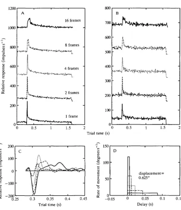
A set of four tests was repeated several times on each neurone studied in this group of experiments (see Materials and methods). The first of these four experiments examined the response of the neurone to impulsive jumps of the image against various adapting background velocities. These results showed that for stimulus repetition rates like those used by Srinivasan (1983) (about 1.5 s, i.e. quite unadapted) the impulse responses of butterfly neurones exhibited a range of behaviours, as illustrated by the impulse responses of three neurones responding to image motion (Fig. 4A,B,C). The responses of the butterfly neurones were, on the whole, narrower than those of the fly HI neurone (cf. Figs 4C and 11B,D). This imphed that the neurones should easily discriminate stimuli with time courses that would be confused by fly HI (Srinivasan, 1983). When adapted to higher image velocities, the responses of all the cells became biphasic (Fig. 4D,E,F); this suggests a newly acquired 'high-pass' frequency characteristic in response to scene oscillations. The change in response shape demonstrates that the cells cannot be considered to have static response properties.

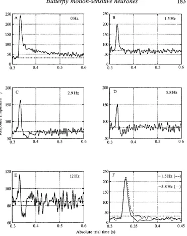
To examine the changes in the response waveform accompanying adaptation in more detail, we summed the responses of five ipsilateral horizontal cells whose responses were nearly indistinguishable. Fig. 5A-E shows the effect on the impulse response of progressively higher adapting velocities. The adapting velocities for each impulse response in Fig. 5 are shown beside each waveform but are expressed as the temporal frequencies generated by moving the 0.2 cycles degree"1 gratings. Thus, 12 Hz corresponds to an angular velocity of 60 degrees s"1. Overall it can be seen that as the adapting velocity increases the impulse responses become narrower and progressively more biphasic. It is necessary to restate here that in each trial the spatial phase of the gratings was shifted so that any afterimage effects (Maddess, 1986) were averaged out. Responses to an impulsive jump in the preferred direction imposed against adapting velocities in the non-preferred direction are also shown (Fig. 5F). Adaptation to a higher velocity in the non-preferred direction (Fig. 5F, solid curve) also appears to narrow the impulse response.

Unadapted

8 0 140

120

100

on 8U

60

40

20

n A

-•

•

v

v •

0.5 1.5

a.

S Adapted

1.6U

110

100

90

80

70

60

vi

D

A

0.5

1ZU

100

on OU

60

40

20

n

B

V

0.5 1.5

0 0.5 1 Absolute trial time (s)

Fig. 4. Velocity impulse responses of three neurones (vertical pairs of panels) in relatively unadapted (A,B,C) and highly adapted (D,E,F) states. In the unadapted state, the cells show a range of behaviours, but when the cells are adapted their responses become similar. For A-C, the only motion was the periodic displacement of the grating every 1.6s by 0.625°. For D-F, in addition to the periodic jumps there was

continuous motion of the 0.2 cycles degree"1 grating at 12 Hz. The cells shown in A,D

and B,E were sensitive to regressive horizontal motion, whereas the cell shown in C and F was sensitive to downward motion. All three were ipsilateral units.

0.6

200

M 150

Q.

100

50"—

0.3 0.4

2.9Hz

0.5 0.6

250 200 150 100 50

0 0.3

Absolute trial time (s) F

A

IV

'•

...L

-1.5Hz(—) -5.8Hz(-)

0.35 0.4 0.45

1200 1000

I"

£

0 0.5 1.5 2 0 0.5

Trial time (s)

1.5

3 Q.

B

Si

£

-- 2 0 0

0.25 0.3 0.35 0.4

Trial time (s)

0.45 1JU 100 50 n D -• -displacement= ', 0.625° 1....

• : > • \ i

-0.05 0.05

Delay (s)

0.1 0.15

frames (see Fig. 6C, dashed curve) is slightly different from the response to a jump of one frame.

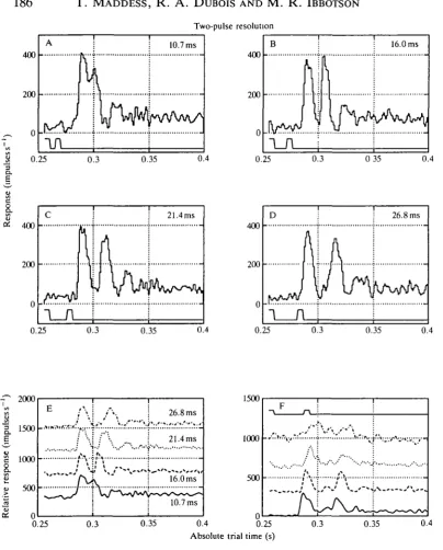
The previous experiments suggest that even in the unadapted state the butterfly neurones should be able to resolve two brief displacements even when they are placed close together. Our third experimental type was thus to measure the 'two-pulse' resolution of these same cells. Responses from a cell where 0.625° displacements were presented with separations of 1, 2, 3 and 4 video frames are given in Fig. 7A-D, respectively. The cell, one of the five whose responses are averaged in Fig. 5, clearly resolves the two displacements even when they are separated by only 16 ms. The responses shown in Fig. 7A-D are replotted together in Fig. 7E for ease of comparison. The responses of four other cells to interdisplacement times of five video frames (32 ms gaps) are shown in Fig. 7F.

Piece-wise linearity

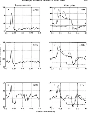
So far little has been said about the ability of the cells to be considered as being piece-wise-linear, i.e. Linear within a given adaptation state. The observation that the responses to pairs of displacements did not differ greatly (Fig. 7 and unpublished data obtained using the drifting dots stimulus) suggests that second-order nonlinearities may not be large. A proof of the concept that the cells could be regarded as piece-wise linear would be the demonstration that responses to more complex stimuli could be predicted by convolution of the velocity kernel. The velocity impulse responses of Fig. 5C,D,E are replotted in Fig. 8A,C,E along with the average responses (Fig. 8B,D,F; dashed curves) of the same cells to repeated stimulation by longer rectangular pulses of velocity superimposed on the same adapting velocities as were used to produce the impulse responses. Shown in solid curves in Fig. 8B,D,F are the predicted responses of these neurones for each adaptation state. The predicted curves are clearly similar to the responses to the longer pulses.

In obtaining the predicted responses the background spike rate was first subtracted from the responses in Fig. 8A,C,E, which were responses to displace-ments of 0.625° in one video frame (5.35 ms). The resulting responses were then scaled by 1/0.625, to model the responses as responses to displacements of 1°; these scaled responses are what we refer to as velocity kernels, and they have units of impulses s"1 degree"1. The kernels were then convolved with the stimulus (having units of degrees s"1) and the original background spike rates were then added back. Perhaps the most interesting feature of the responses is the suggestion from the impulse response of Fig. 8E that the d.c. gain of the system when adapted to 12Hz stimulation would be almost 0. This prediction arises because, with the background subtracted, the area under the response of Fig. 8E is almost 0 and the gain of a linear system at OHz is exactly equal to the area under the kernel (see Fig. 12, Discussion). Following this prediction, the response of the cell in Fig. 8F to the plateau of the velocity pulse (OHz) is almost equal to the steady-state Response, i.e. no response.

Two-pulse resolution

is

400 f n4 1 I 400

-3 a.

I

in

0.3 0.35 0.4

c

1

flj

1

i_n

i

16.0 ms

0.3 0.35 0.4

400

200

0

-0.25

0.3 0 35 0.4

D

A

i n

26.8 ms

0.3 0.35 0.4

~ 2000

1500 H

a

1000

u 500 -E

# t.j

f

!>*.... "

26.8 ms 21.4ms

"16.0 m s " 10.7 ms

0

0.25 0.3 0.35 0.4 0.25

Absolute trial time (s) 1000 500 0 F rv •/.*•'. i\ i ,••• ; \

'"h

f\~

^ \ /

Fig. 7. The integration time of a relatively unadapted cell assessed by varying the distance between two temporally adjacent jumps. At a separation of 16 ms (B) the two pulses are clearly resolved, showing that the integration time is less than 20 ms. The time course of the jumps is indicated by the rectangular trace below each response. (E) The four responses of A-D plotted together to aid comparison. (F) Responses of the four other cells shown in Fig. 5 to a pair of 0.625° jumps displaced by 32 ms. A-D are the averages of at least 128 repetitions.

187

200

1 5 0

100 -50 0.3 Impulse responses A

J

1 ! 1

| | | 2.9Hz

0.35 0.4 0.45 0.5

100 90 70 -60 0.3 0.35 Weber pulses B _.',

•r

•i

j

0.4 0.45 0.5

200

1 150 -| E 100 -50 0

c

r

-3 0.-35 0.4 0.45 0.5 60

D _:\

tt

...A... /'

s * / *

0.3 0.35 0.4 0.45 0.5

120 100 -60 E

J

J

vv

-50' ' • ' 1 60 0.3 0.35 0.4 0.45 0.5 0.3

Absolute trial time (s)

F

A

\

o i l ••

\A

-\ if

1/

-—\fi--^

12 Hz

0.35 0.4 0.45 0.5

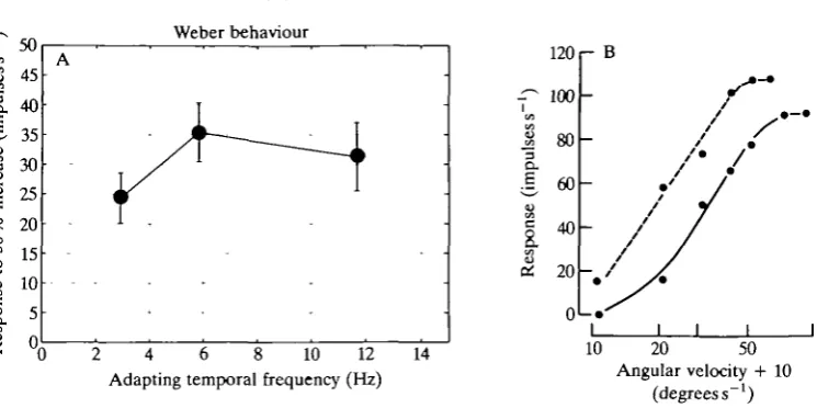
gain, or scale, of the responses to the longer pulses is also well predicted by convolution of the stimulus with the velocity kernels. This is demonstrated by the observation that the amplitudes of the velocity increments used in the experiments of Fig. 8B,D,F were very different but the amplitudes of the responses were, nevertheless, well matched by the predictions. The different amplitudes of the velocity pulses were used because a secondary purpose of the test pulses used in experiments like those of Fig. 8B,D,F was to investigate whether the neurones encode velocity relative to the mean background velocity. That is, the long velocity pulses were designed to test whether the neurones exhibit Weber's law (equation 2) which was our fourth velocity adaptation experiment. In the experiments of Fig. 8B,D,F, the amplitude of the velocity increments was in each case 50 % higher than the background adapting velocity. If Weber's law were to operate, then the cell's responses to the 'Weber' test pulses should reflect the relative velocity, i.e. cells would encode the percentage difference in the velocity of the pulse relative to the adapting velocity rather than the absolute velocity. Similar behaviour in fly lobula plate neurones has also been demonstrated (Maddess and Laughlin, 1985).

Weber's law states that:

&:(AStimulus) , „ AResponse = — , (2)

Stimulus

where a change in the response or the stimulus is indicated by a capital delta, the bar over the quantity in the denominator indicates an average and A: is a constant. A system obeying Weber's law gives a constant-sized response to all stimuli that are the same fraction of the mean stimulus.

Fig. 9A summarises the responses of five cells whose responses to a 50% increase in stimulus velocity were obtained for three background velocities each an octave apart. The responses are not significantly different, indicating that Weber's law roughly holds and that the cells, when adapted, respond to relative velocity rather than to absolute velocity. The data of Fig. 9A only demonstrate that Weber's law works for 50 % increments. It would be instructive to show that the gain control works at a variety of other velocities as well. Experiments were, therefore, carried out on one other horizontal cell.

189

Weber behaviour

120 ~ 100

i - B

80

60

40

2.

oi 20 0

2 4 6 8 10 12 Adapting temporal frequency (Hz)

14 10 20 50

Angular velocity + 10 (degrees s"1) Fig. 9. If the cells were to obey Weber's law, the response to percentage deviations from the different adapting velocities would be the same, i.e. the cells would only encode relative velocity. The data are those of Fig. 8B,D,F replotted against adapting temporal frequency. (A) Despite the fastest stimulus (17.5 Hz or 87.6 degrees s"1) being four times faster than the slowest one (4.4Hz or 22 degrees s"1), the cells respond to the percentage change, i.e. their responses to 50% velocity increments are not significantly different. Error bars are standard deviations of five cells' responses. (B) To achieve Weber's law, a simple multiplicative change in gain is required between adaptation states. The lateral shift between the unadapted (dashed) and adapted (solid) curves indicates such a multiplicative gain change. The adapting velocities were 0 (dashed line) and 34 degrees s"1 (solid line). The shift means that while the cell responds less well to small velocities when adapted it, nonetheless, gives better response modulation to changes in velocity centred on 40 degrees s"1. Each point in B is the average of 200 trials and the 95 % confidence limits on each value are smaller than the symbols. The responses were obtained in random order. The abscissa is given as 'angular velocity+10' to allow the response to 0degreess~l, i.e. the background spike rate, to be shown.

indicated by the reduced dynamic range is probably more than offset by the increase in temporal resolution that was also observed. The shift is thus analogous to that seen in photoreceptors on adaptation to higher average light levels and which leads to the encoding of image contrast (e.g. Laughlin and Hardie, 1978). Some information about absolute velocity is retained in the cells in the form of their steady-state spike rate. Consistent with results obtained in the fly HI neurone (Maddess and Laughlin, 1985), the steady-state spike rate increases with increas-ing adaptation state, providincreas-ing some indication of the absolute velocity but on a very slow time scale. Therefore, in adapting, the cells appear to be sacrificing information about the absolute velocity in return for higher temporal resolution of rapid motion. Also consistent with results from the fly (Zaagman et al. 1983) was the finding (not shown) that neither the time to peak nor the delay of the impulse ^responses appears to contain any significant information about the background

Frequency response

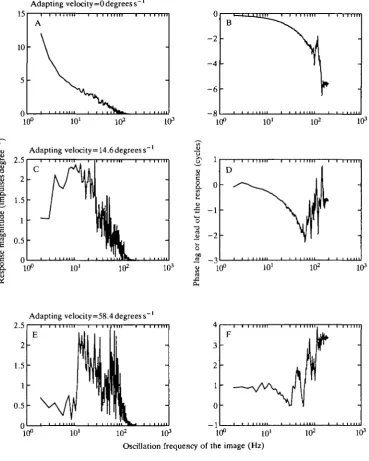
Since the data of Figs 8 and 9 indicate that the cells may be thought of as being piece-wise linear, it is therefore reasonable to examine the Fourier transforms of the velocity kernels to assess the effects of adaptation on the temporal frequency response of the neurones. The reader should keep in mind that the frequencies referred to here are frequencies of back-and-forth oscillations of a scene rather than contrast frequency. The velocity kernels suggested that, with adaptation to higher velocities, there is a diminution of the representation of lower temporal frequencies. Fig. 10A,C,E shows the Fourier transforms of the velocity kernels derived from Fig. 5A,C,E. The responses indicated by the ordinate represent the predicted response of the cell in each of the three adaptation states to oscillation of the test scene by a sinusoidal time-varying velocity having an amplitude of 1 degrees"1. For example, Fig. IOC indicates that when the cell has been adapted to a mean image velocity of 14.6 degrees s- 1 the response to a further 10 Hz oscillation of the scene of amplitude 1 degree s"1 would be a response modulation of about 2.5 impulses s"1. An interesting feature of Fig. 10A,C,E is that whereas the response to low frequencies diminishes with adaptation, the gain of the high-frequency response, from 10 to 100Hz, hardly changes at all (note that the ordinate scale in Fig. 10A differs from that in Fig. 10C,E).

Other stimuli

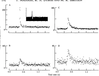
A possible criticism of the previous experiments is that the responses were for the most part to sinusoidal gratings (note the exception of Fig. 9B). It would be instructive to explore other more general stimuli to see whether the adaptive properties described above are an artefact of stimulation with periodic patterns or some other such effect. To this end, some responses were obtained to moving fields consisting of drifting dots (see Materials and methods). As in the impulse response experiments described above, the stimuli were single displacements of the field of dots presented against a range of adapting drift velocities. As the excitatory phases of the impulse responses were already very narrow, even in relatively unadapted conditions, the best indication of variations in temporal tuning proved to come from the inhibitory phases of the impulses responses obtained under adaptation in continuous motion. The responses obtained in these experiments (not shown, but see fly experiments below) were very similar to those of Fig. 4, which were obtained with gratings. Other experiments, such as those of the integration time experiments of Figs 6 and 7, were also repeated with the drifting dot stimuli and the results were in agreement with those obtained with gratings.

Comparison with flies

191

Adapting velocity=0 degrees s

Adapting velocity=14.6degrees s

3 Q.

B

8.

Adapting velocity=58.4 degrees s

10 102 103 10° 10'

Oscillation frequency of the image (Hz)

Fig. 10. Amplitude spectra (A,C,E) and phase shifts (B,D,F) for velocity kernels derived from Fig. 5A,C,E. Notice that the gain of the higher frequencies appears to change little, while the gain of the low frequencies of image oscillation is reduced by about 20 times.

I - A

200

O1

-180r- C

o1

-3 D.

e

8

i

01

-9 0 r - D

' * • ' .

-01

-0.0 0.6 1.2 0.0

Trial time (s)

0.6 1.2

Fig. 11. Velocity impulse responses of a sample of Lucilia cuprina lobula plate cells obtained with the random dot pattern (see Materials and methods). (A) Response of a vertical cell to downward jumps (inset, the response of the same cell with adaptation to

constant motion at 20 degrees s"1). (B,C) The unadapted responses of two HI cells are

in agreement with previous results obtained with gratings. (D) A cell sensitive to downward motion. (A,B,D) Responses to single-frame (6.57ms) displacements (jumps) of the field of dots by 0.83°; (C) the response to jumps of 0.42°.

according to the nomenclature of Hausen (1976). Some cells sensitive to downward motion (e.g. Fig. 11D) and some HI neurones (Fig. 11B,C) showed much broader velocity impulse responses. The results for the fly HI neurones accord with results obtained with grating stimuli here and elsewhere (Srinivasan, 1983; Zaagman et al. 1983). Thus, it would appear that the responses of fly lobula plate neurones to the two-dimensional dot stimulus are, as expected, similar to those induced by gratings.

Discussion

Bipolar responses

cell to code the other stimulus polarity. However, half-wave rectification and the use of two cells to code a signal might make sense because such a scheme constitutes a form of range fractionation. By having two or more cells, each with a limited information capacity, share the responsibility of responding to a given stimulus dimension, the ability of each cell to represent fine changes in the stimulus is enhanced. The high background spike rates of the neurones described here do not appear to be due to adaptation because they can occur when even relatively unadapting stimuli, such as slowly drifting lines, are used (e.g. Fig. 2A,E).

Contrast sensitivity functions

It was pointed out in the Results section that the spatial frequency tuning of medulla neurones was more consistent with receptive fields the size of photorecep-tors than the large fields displayed in Fig. 2A,C,E. This statement arises from the fact that there is a spatial equivalent for equation 1 which says that broad spatial frequency tuning requires a narrow receptive field envelope, i.e. tuning widths and receptive field envelopes are reciprocally related (see Geisler and Hamilton, 1986, for a discussion). The broad spatial tuning shown in Fig. 3A,B is, therefore, not consistent with the broad receptive fields of Fig. 2A,C,E, but instead is indicative of receptive field sizes close to those of photoreceptors. It has recently been pointed out that the nonlinear process of motion detection will preserve the spatial frequency tuning of presynaptic units (Egelhaaf and Borst, 1989), and so we conclude that the spatial tuning observed in Fig. 3A,B represents that of units presynaptic to the motion-detection process.

One conspicuous difference between the threshold spatial frequency tuning curves of Papilio aegeus and those of the HI neurone of Lucilia cuprina (Dvorak et

al. 1980) is the steep low-frequency roll-off of the Papilio cells, even at high

temporal frequencies. In particular, fly HI cells show no roll-off at 10 Hz. Dvorak

et al. (1980) and Srinivasan and Dvorak (1980) took the lack of roll-off as an

indication that the temporal frequency response of spatially flanking inhibitory zones around the subunit receptive fields was exceeded. This could indicate that in the butterfly the lateral inhibition is not as sluggish as it is in the fly. This, in turn, may be related to the observation that, overall, the unadapted temporal acuity of the butterfly medulla neurones seemed to be somewhat higher than that of fly lobula plate neurones.

influence of spatially flanking inhibitory zones when, in fact, they are not (Reichardt and Schogl, 1988). If this effect also explains the low-spatial-frequency roll-off in the butterfly, the butterfly elementary motion detectors are obviously somewhat different from their counterparts presynaptic to fly lobula plate neurones.

On adaptation and velocity kernels

Why should direction-selective neurones adapt at all? The answer lies in the finite number of just-discriminable responses that a neurone can generate. When the number of just-discriminable states available is small compared to the requisite decision time, the neural system may be forced to sacrifice some information so that essential data are not lost. The response time of acrobatic insects, such as butteflies and flies, in flight is approximately 30ms (Land and Collett, 1974; Wehrhahn, 1984). At the same time, the information capacity of neurones like those studied here is about 90 bits s~* (de Ruyter van Steveninck and Bialek, 1988). In one reaction time the neurone could convey about 6.5 (=29 O x 0 0 3) just-discriminable response states on which to base its flight correction. To put this in its proper perspective, one must understand that insects give accurate, graded, optokinetic responses to stimuli moved to produce contrast frequencies from as low as 0.2 Hz to as high as 200Hz (McCann and MacGuinite, 1965). If the optokinetic neurones responded linearly to this range of frequencies one is left with the absurd prospect of reconciling animals that can produce fine optokinetic tracking at contrast frequencies of 0.2Hz with neurones that cannot discriminate changes of contrast frequency smaller than 30 Hz (=200/6.5). The present work provides evidence that the dilemma is resolved by an adaptive process that modifies the neurones' gain and temporal tuning to match motion signals distributed about the current mean motion signal. Thus, the motion-sensitive neurones studied here exhibit rough adherence to Weber's law and, in so doing, spread their limited response states to span the prevailing distribution of motion signals (cf. Laughlin, 1981, on encoding image contrast distributions).

adaptation state and, finally, that complete recovery from even a few seconds of continuous motion could take over 10 s.

The two groups then proceeded to measure different aspects of the effects of image motion. Maddess and Laughlin (1985) examined what determined the rate of response decay to continuous motion, whereas de Ruyter van Steveninck et al. (1986) examined the effects of continuous motion on the time constant of the velocity impulse response. An important difference in these studies was that Maddess and Laughlin (1985) did not use stimulus temporal frequencies much below 2 Hz and found that response decline depended on temporal frequency rather than on velocity, de Ruyter van Steveninck et al. (1986) found that below 2 Hz the time constant of the velocity impulse response was a function of stimulus velocity rather than stimulus temporal frequency. Maddess and Laughlin (1985) avoided the low temporal frequency region because of the presence of afterimage effects at these frequencies (Maddess, 1986).

Thus, the differing conclusions about what governs adaptation may reflect the different temporal frequency domains used. It is possible that when average image velocities are slow a scheme like that recently proposed by Reichardt et al. (1988) could calculate the absolute image velocity. At high image velocities, this may be too time consuming or unnecessary, given that adaptation means that only relative velocity signals are available anyway. Thus, the factor governing adaptation levels may switch from the veridical image velocity to relative measures such as temporal frequency at high image velocities. Interestingly, a temporal-frequency-dependent adaptation mechanism also operates in direction-selective cells of the cat visual cortex (Maddess et al. 1988; Bonds, 1991).

In a more recent study of adaptation of the velocity impulse response of lobula plate neurones, Borst and Egelhaaf (1987) have confirmed that even temporal modulation of luminance, in the absence of a motion signal, adapts HI and other lobula plate neurones. Maddess and Laughlin (1985) also reported this but maintained that moving stimuli were more effective at adapting HI than flicker at the same temporal frequency. Maddess and Laughlin's (1985) evidence was again based on the rate of response to steady stimulation while Borst and Egelhaaf (1987) examined the time constant of the velocity impulse response. They concluded that flicker changed the neurone's time constant almost as much as motion.

200

Area=6 impulses

a.

B Area=l impulse

0.05 0.1 0.15

Delay (s)

0.2

Scene oscillation rate (Hz)

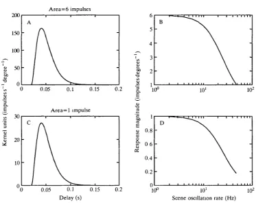
Fig. 12. Hypothetical velocity kernels (A,C) and their Fourier transforms (B,D) indicate the effect on response gain of the area of the velocity kernel and how this effect is independent of the time constant of the kernel. The area of two 'low pass' kernels which have similar time courses completely determines the relative gain of all the frequencies and is exactly equal to the gain at OFfz.

similar amount. To examine a more concrete example, the area under the impulse response of Fig. 5E is nearly zero and the gain at OHz and nearby frequencies is very small (Fig. 10E).

In Borst and Egelhaaf s (19S7) results the time constants of the impulse derived for 4 Hz motion and 4 Hz flicker were similar, but the magnitudes and areas of the two impulse responses were quite different. An examination of these areas indicates that the response of the HI neurone to velocity modulations, when adapted to 4Hz motion, would be expected to result in response modulations six times smaller than those produced by adaptation to 4 Hz flicker. This ratio of the expected gains arises because the ratio of the areas of the impulse responses for these two adapting conditions is 6, just as in the example of Fig. 12. Therefore, it would appear that although the time constant of the velocity kernel is set by the flicker rate the overall gain may be determined by the extent to which the stimulus is dominated by motion or flicker.

The spatial frequency tuning is very similar in horizontal and vertical cells, indicating that similar small-field units are presynaptic to both. Threshold temporal tuning curves are also similar for both horizontal and vertical cells, once again suggesting similar subunit structure. Intracellular recordings reported on elsewhere (Ibbotson et al. 1991) indicate that the neurones reported on here are large medulla neurones.

Papilio neurones show signs of very high temporal resolution of changes in

image velocity, even in the unadapted state. In particular, relatively unadapted units could resolve differences in the time course of stimuli (Fig. 6A,B) that a similarly adapted fly HI neurone could not discriminate as being different (Fig. 11B,C; Srinivasan, 1983). Also, pairs of velocity impulses are easily discriminated, even when separated by only 16ms (Fig. 7B). These observations, taken in conjunction with the lack of significant facilitation or inhibition of responses to pairs of impulses (i.e. no indication of significant second-order nonlinearities), suggest that the use of velocity impulse responses provides a reasonable estimate of the cell's ability to resolve changes in image motion. The fact that responses to more complex stimuli could be predicted by convolution with velocity kernels measured for particular adaptation states reinforces the idea that the cells can be thought of as being wise linear. The conclusion of piece-wise linearity is further reinforced by the fact that the stimuli used to obtain the velocity kernels were strong: if significant nonlinearities were present they should manifest themselves in response to powerful stimulation. Overall, the gradual transition to biphasic responses with increasing adaptation to motion is suggestive of a strategy similar to predictive coding (Srinivasan et al. 1982).

The Papilio neurones also appear to show adaptive characters similar to those of lobula plate units in flies. Like the fly neurones (de Ruyter van Steveninck et al. 1986; Borst and Egelhaaf, 1987) adaptation was also observed to stimuli moved in the non-preferred direction (Fig. 5F). Also like fly lobula plate cells, evidence is provided that adaptation means that the cell's response does not encode absolute image speed but, instead, velocity relative to the recent stimulus history, which has been called 'velocity contrast' (Maddess and Laughlin, 1985) because of the similarity between this process and the compression of light intensity into luminance contrast by photoreceptors (e.g. Laughlin and Hardie, 1978).

We would like to thank A. James, S. Marcelja and M. V. Srinivasan for helpful discussions.

References

BONDS, A. B. (1991). Temporal dynamics of contrast gain in single cells of the cat striate cortex.

Visual Neurosci. 6, 239-255.

BORST, A. AND EGELHAAF, M. (1987). Temporal modulation of luminance adapts time constant of fly movement detectors. Biol. Cybernetics 56, 209-215.

COLLETT, T. (1971). Connections between wide-field monocular and binocular movement detectors in the brain of a hawk moth. J. comp. Physiol. 75, 1-31.

COLLETT, T. (1972). Visual neurons in the anterior optic tract of the privet hawk moth. J. comp.

Physiol. 78, 396-433.

COLLETT, T. AND BLEST, A. D. (1966). Binocular directionally selective neurons, possibly involved in the optomotor response of insects. Nature 212, 1330-1333.

DE RUYTER VAN STEVENINCK, R. AND BIALEK, W. (1988). Real-time performance of a movement-sensitive neuron in the blowfly visual system: coding and information transfer in short spike sequences. Proc. R. Soc. B 234, 379-414.

DE RUYTER VAN STEVENINCK, R. R., ZAAGMAN, W. H. AND MASTEBROEK, H. A. K. (1986). Adaptation of transient responses of a motion-sensitive neuron in the visual system of the blowfly Calllphora erythrocephala. Biol. Cybernetics 54, 223-236.

DVORAK, D., SRJNIVASAN, M. V. AND FRENCH, A. S. (1980). The contrast sensitivity of fly motion-detecting neurons. Vision Res. 20, 397-407.

EGELHAAF, M. AND BORST, A. (1989). Transient and steady-state response properties of movement detectors. J. opt. Soc. Am. A6, 116-127.

GEISLER, W. S. AND HAMILTON, D. B. (1986). Sampling theory analysis of spatial vision. J. opt.

Soc. Am. A3, 62-70.

HAUSEN, K. (1976). Functional characterisation and anatomical identification of motion sensitive neurons in the lobula plate of the blowfly Calllphora erythrocephala. Z. Naturforsch. 31c, 629-633.

HOWARD, J., DUBS, A. AND PAYNE, R. (1984). The dynamics of phototransduction in insects. A comparative study. J. comp. Physiol. 154, 707-718.

IBBOTSON, M. R., MADDESS, T. M. AND DUBOIS, R. A. (1991). A system of insect neurons sensitive to horizontal and vertical image motion connect the distal medulla and midbrain.

J. comp. Physiol. (in press).

KIRSCHFELD, K. (1989). Automatic gain control in movement detection of the fly.

Naturwissenschaften 76, 378-380.

LAND, M. F. AND COLLETT, T. S. (1974). Chasing behaviour of houseflies (Fannia canicularls).

J. comp. Physiol. 89, 331-357.

LAUGHLIN, S. B. (1981). A simple coding procedure enhances a neuron's information capacity. Z. Naturforsch. 36c, 910-912.

LAUGHLIN, S. B. AND HARDIE, R. C. (1978). Common strategies for light adaptation in the peripheral visual systems of fly and dragonfly. J. comp. Physiol. 128, 319-340.

MADDESS, T. (1986). Afterimage-like effects in the motion-sensitive neuron HI. Proc. R. Soc. B 228, 433-459.

MADDESS, T. AND LAUGHLIN, S. B. (1985). Adaptation of the motion-sensitive neuron HI is generated locally and governed by contrast frequency. Proc. R. Soc. B 225, 251-275.

MADDESS, T., MCCOURT, M. I., BLAKESLEE, B. AND CUNNINGHAM, R. B. (1988). Factors governing the adaptation of cells in area-17 of the cat visual cortex. Blol. Cybernetics 59, 229-236.

MASTEBROEK, H. A. K., ZAAGMAN, W. H. AND LENTING, B. P. (1980). Movement detection: performance of a wide-field element in the visual system of the blowfly. Vision Res. 20, 467-474.

MCCANN, G. D. AND MACGUINITE, G. F. (1965). Optomotor response studies of insect vision.

Proc. R. Soc. B 163, 369-401.

MERRILL, E. G. AND AINSWORTH, A. (1972). Glass coated platinum-plated tungsten microelectrodes. Med. Blol. Eng. 10, 662-667.

MILDE, J. J. (1988). Neuronal basis of visually guided behaviour in Manduca sexta. Proc. 16th

Neurobiol. Conf. 232.

PAYNE, R. AND HOWARD, J. (1981). Response of an insect photoreceptor: a simple log-normal model. Nature 290, 415-416.

REICHARDT, W. (1961). Autocorrelation, a principle for the evaluation of sensory information by the central nervous system. In Principles of Sensory Communication (ed. W. A. Rosenblith), pp. 303-307. New York: Wiley.

derived from behavioural experiments on the visual system of the fly. Biol. Cybernetics 58, 287-294.

REICHARDT, W. E. AND GUO, A. (1986). Elementary pattern discrimination (behavioural experiments with the fly Musca domestica). Biol. Cybernetics 53, 285-306.

REICHARDT, W. E. AND SCHLOGL, R. W. (1988). A two dimensional field theory for motion computation. First order approximation; translatory motion of rigid patterns. Biol.

Cybernetics 60, 23-35.

REICHARDT, W. E., SCHLOGL, R. W. AND EGELHAAF, M. (1988). Movement detectors provide sufficient information for local computation of 2-D velocity field. Naturwissenschaften 75, 313-315.

RIND, C. F. (1983a). A directionally sensitive motion detecting neuron in the brain of a moth. /. exp. Biol. 102, 253-271.

RIND, C. F. (1983ft). The role of an identified brain neuron in mediating optomotor movements in a moth. /. exp. Biol. 102, 273-284.

SRINIVASAN, M. V. (1983). The impulse response of a movement-detecting neuron and its interpretation. Vision Res. 6, 659-663.

SRINIVASAN, M. V. AND DVORAK, D. R. (1980). Spatial processing of visual information in the movement detecting pathway of the fly. /. comp. Physiol. 140, 1-23.

SRINIVASAN, M. V., LAUGHLIN, S. B. AND DUBS, A. (1982). Predictive coding: a fresh view of inhibition in the retina. Proc. R. Soc. B 216, 427-459.

SWIHART, S. L. (1969). Colour vision and the physiology of the superposition eye of a butterfly.

J. Insect Physiol. 15, 1347-1365.

WEHRHAHN, C. (1984). Visual orientation of flies in flight. In Localization and Orientation in

Biology and Engineering (ed. D. Varju and A. Schitzler), pp. 113-118. Berlin:

Springer-Verlag.

ZAAGMAN, W. H., MASTEBROEK, H. A. K. AND DE RUYTER VAN STEVENINCK, R. (1983). Adaptive strategies in fly vision: on their image-processing qualities. IEEE Trans. SMC 13, 900-906. ZAAGMAN, W. H., MASTEBROEK, H. A. K. AND KUIPER, J. W. (1978). On the correlation model:

performance of a movement detecting neural element in the fly visual system. Biol.