SANTOSS sand transport model: Implementing and testing within the morphological model UNIBEST TC

(1)

SANTOSS sand transport model:

Implementing and testing within the

morphological model UNIBEST-TC

(2)

(3)

15th March 2011, final report

SANTOSS sand transport model:

Implementing and testing within the

morphological model UNIBEST-TC

Enschede, 15th March 2011

This master thesis was written by Harm Gerrit Nomden

As fulfillment of the Master’s degree Civil Engineering & Management University of Twente, The Netherlands

Under supervision of the following committee Dr. Ir. J.S. Ribberink

Dr. Ir. J. J. Van der Werf Ir. W. M. Kranenburg

(4)

(5)

Title

SANTOSS sand transport model: Implementing and testing within the morphological model UNIBEST-TC

Client Deltares

University of Twente

Pages

Main report: 70 Appendices: 35

(6)

(7)

Abstract

Due to the large (and increasing) amount of activities in coastal areas, predictions of the short-term and long-term morphological developments are becoming more and more important to ensure safety, navigation, recreation and ecology. To make these morphological predictions different modelling systems are developed including several sand transport formulations.

Recently, a new sand transport model was released by Ribberink et al. (2010), as a result of the research project SANTOSS (SANd Transport in Oscillatory flows in the Sheet-flow regime),. The model describes the sand transport within the wave boundary layer under (1) non-breaking waves with different shapes; (2) waves combined with currents; (3) for a large range of sand grain sizes; and (4) for both the ripple and sheet flow regime. The model is calibrated on detailed experiments in oscillatory flow tunnels and wave flumes and it explicitly accounts for unsteady (phase lag) and wave non-linearity effects (skewed and asymmetric waves) and for additional processes under real waves (e.g. boundary layer streaming, Lagrangian effects and vertical orbital velocities. Based on experiment results the SANTOSS sand transport model seems to predict the measured transport rates better in comparison with other transport models. The goal of this research is to explore the applicability and behaviour of the SANTOSS transport model within a morphological model. This has been done by implementing the SANTOSS model within the morphological model UNIBEST-TC and comparing the results of a sensitivity analysis and two test cases with measurements and the results from the TRANSPOR2004 (TR2004) transport model, which was already implemented

(Van Rijn, 2007a, 2007b).

The SANTOSS model was implemented successfully in the cross-shore profile model UNIBEST-TC. Some small adjustments to the SANTOSS code were necessary to make it more robust. Additionally, special attention is paid to the generation of representative orbital velocity time series which show both velocity skewness and acceleration skewness. Therefore, different theories are analyzed, tested and combined. Because the SANTOSS model does not cover the transport above the wave boundary layer, the current-related suspended load transport at higher levels is computed using the TR2004 formulations.

The sensitivity analysis focused on (1) predicted net transport rates and (2) the influence of several processes on the transport. It showed that the SANTOSS model reacts almost in the same way as the bed load and wave-related suspended load of TR2004 together. With the only difference that transport rates predicted by the SANTOSS model are lower over the whole range. In the ripple regime the transport rates predicted by SANTOSS are reduced to zero or become even slightly negative, mainly due to phase lag effects. The TR2004 model predictions are also almost reduced to zero when a phase lag factor is applied to the wave-related suspended load. In the sheet flow regime the increasing undertow velocity near the bed (due to partially breaking waves) and enhanced suspended sediment generate a high offshore directed current-related suspended load, which becomes dominant for both transport models. The influence of different transport and hydrodynamic processes within the two transport models, like phase lag, acceleration and surface wave effects (only for the SANTOSS model) are analysed. Also influences of breaking waves and the use of different orbital velocity theories are explored for both models. Main conclusions are:

(8)

25 January 2011, final report

 Phase lag effects and surface wave effects (especially vertical orbital velocities) are of importance in the ripple regime. In the higher sheet flow regime the relative influence is low, because it is totally dominated here by the current-related suspended load.

 Acceleration effects are taken into account in a different way by the two transport models and has much more influence on the TR2004 predictions;

 The level from which the superimposed mean current velocity is extracted as input for the bed load transport is of large importance. The two transport models use a different level. This was shown to have a significant influence on the predicted transport rate.

To assess the performance of the two transport models on predicting morphological evolution, two test cases are used: LIP IID test 1B (erosive conditions, sand bar development) and test 1C (accretive conditions, onshore sand bar migration). For test 1B, modeled hydrodynamics agree in general well with measurements, but modeled concentrations of suspended sediment are overestimated offshore of the bar. Both transport models show a weak sand bar development and too much offshore bar migration (SANTOSS slightly more than TR2004). For test 1C there is some differences in modeled and measured hydrodynamics: velocity skewness of the orbital velocities and the undertow velocity in the trough onshore of the sand bar. This also explains the bad performance in morphological predictions by both transport models: small offshore bar migration instead of clear onshore migration.

(9)

Preface

This thesis represents the work that has been carried out at Deltares for my Master thesis project, relating the prediction of sand transport under coastal conditions by two transport formulations in a coastal morphological model. I really liked working with theories and models and it is something in I want to keep doing in the future, although it has also brought a lot of standard modelling frustration about theories that are hard to understand, are not perfectly implemented, do not work well in a specific case, the large uncertainties in this complicated modelling field and off course the endless debugging (also due to my own mistakes).

First, I would like to thank my three supervisors Jan, Jebbe and Wouter for introducing me in the world of sand transport, their interest in my work and their useful comments on my work. Especially my daily supervisor Jebbe, who I could interrupt at anytime, to discuss every strange topic or problem I had on my mind. I hope my work have contributed to their work and knowledge.

Next, I’m really grateful to have worked at Deltares, which gave me the opportunity to meet interesting and smart people and who gave me access to a tremendous amount of knowledge about hydrodynamic and sand transport modelling and coastal models. I would like to thank the people at the unit Marine and Coastal Systems and also Dirk Jan Walstra for answering the questions I had about the modelling and simulating part. I also want to thank Mr. Abreu for borrowing his code on wave form definition, which helped me a lot during my research.

I want to thank my fellow students at Deltares: Peter, Martijn, Sanne, Ingrid, Jorik, Rik, Kees, Giorgio (sorry again for calling you a student), Arnold, Brice and the students at Hydraulic Engineering for keeping me from my work, drinking coffee, chatting around and also discussing serious topics (football). Also I like to thank my housemates in Delft and in Enschede (sorry for the stress I brought home) and my friends of Pallet # for the great 7.5 years and for the phone calls when they were stuck in a traffic jam from work. Last but not least, I thank my parents and brothers and especially my girlfriend Lianne for her contribution to my work, good advices, love and lots of encouragements.

I hope you will enjoy reading this report.

Harm Nomden

(10)

(11)

Content

1. Introduction 1

1.1. Context 1

1.2. Research definition 2

1.3. Research questions and methodology 2

2. Research background 5

2.1. Introduction 5

2.2. Hydrodynamic aspects 5

2.2.1. Wave propagation 5

2.2.2. Orbital motion 5

2.2.3. Currents 7

2.2.4. Boundary layer flow 7

2.3. Sediment transport aspects 7

2.3.1. Sediment properties 7

2.3.2. Transport regimes in oscillatory flow 8

2.3.3. Bed shear stress and wave form effects 8

2.3.4. Unsteady effects in oscillatory flow 9

2.3.5. Influence surface wave effects on sediment transport 9

2.4. Morphological aspects and modelling 9

2.5. Conclusions 10

3. Model descriptions 11

3.1. Introduction 11

3.2. UNIBEST-TC 11

3.2.1. Wave propagation module 11

3.2.2. Mean current profile module 12

3.2.3. Near bed orbital velocity module 12

3.2.4. Sediment transport module 12

3.2.5. Bed level change module 12

3.3. Two practical sediment transport models 12

3.3.1. TRANSPOR2004 sand transport model 13

3.3.2. SANTOSS sand transport model 15

3.3.3. Performance transport models (previous research on comparison

transport predictions with experiment data) 17

3.4. Conclusions 18

4. Implementation SANTOSS model in UNIBEST-TC 19

4.2. The SANTOSS sand transport code 19

4.3. Influence of bed-slopes on sediment transport 21

4.3.1. Slope effect on threshold of sediment transport 22 4.3.2. Slope effects on the transport rates and the direction 22 4.3.3. Including slope effects in SANTOSS formulations in UNIBEST-TC 23

4.4. Short wave flow velocity 24

4.4.1. Analysis available theories 25

4.4.2. Application SANTOSS in UNIBEST-TC 27

4.5. Wave group effect on near bed orbital velocity 29

4.5.1. Current application in UNIBEST-TC 29

(12)

4.6. Superimposed current 30

4.6.1. Current application in UNIBEST-TC 30

4.6.2. Application SANTOSS in UNIBEST-TC 31

4.7. Suspended load transport above wave boundary layer 31

4.8. Conclusions 32

5. Sensitivity analysis transport models within UNIBEST-TC 33

5.2. Set-up and standard settings 33

5.3. Model behaviour 34

5.3.1. Hydrodynamic exploration 36

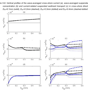
5.3.2. Grain size variation 36

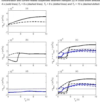
5.3.3. Wave period variation 38

5.3.4. Wave height variation 40

5.4. Comparison between orbital velocity theories 42

5.5. Conclusions 45

6. Application of SANTOSS model to test cases 47

6.2. Description LIP IID experiments 47

6.3. Hydrodynamic calibration 47

6.4. Transport predictions and morphology 50

6.5. Conclusions 51

7. Conclusions, discussion and recommendations 63

7.2. Conclusions 63

7.3. Discussion 65

7.4. Recommendations 66

8. References 69

List of Symbols 73

List of Figures and Tables 75

A. UNIBEST-TC with TR2004 and SANTOSS 1

A.1. UNIBEST-TC: General user-defined input and boundary conditions 1

A.2. UNIBEST-TC: Wave module 3

A.3. UNIBEST-TC: Current profile module 7

A.4. UNIBEST-TC: Orbital velocity module 12

A.5. UNIBEST-TC: Sediment transport modules 14

B. Different orbital velocity theories 23

B.1. Current options and proposed changes to orbital velocity module 23

B.2. Analysis formula Abreu et al. (2010) 23

B.3. Generation of necessary wave form parameters 27

(13)

1.

Introduction

This research focuses on the implementation and testing of the new SANTOSS sand transport model in the coastal morphologic modelling system UNIBEST-TC. This chapter describes the research objective, research framework and the research questions, but first provides a short context of the research.

1.1. Context

Due to the large (and increasing) amount of activities in coastal areas, it is becoming more and more important to be able to predict short-term and long-term morphological developments in coastal areas and to increase knowledge of important hydrodynamic and sand transport processes. Points of interest are for example the development of the coastline, the impact of sea level rise on coastal development, the design of sea harbours, the planning and design of sand nourishment schemes to protect the land and other coastal defence measures or policies in order to the conserve or protect the coastal environment and ecosystem.

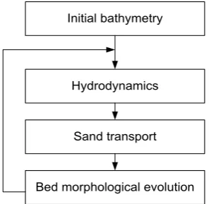
The transformation of waves, local currents, and the resulting sediment transport in the nearshore depend strongly on the bathymetry. If sediment flux gradients modify this bathymetry (e.g., onshore or offshore sandbar migration), subsequent wave and current patterns change as well. This, in turn, leads to further modifications of the bathymetry (See Figure 1-1). The complexity lies in the prediction of the strong variability in time and space and the feedback between the processes.

Morphological modelling systems are used to compute the hydrodynamics and the resulting sediment transport and morphological evolution. Field and lab research during the last decades resulted in better knowledge of waves and currents and their (combined) influence on the sand transport. Based on this knowledge more accurate practical sand transport models were developed. The current state of the art sand transport model is TRANSPOR2004 (Van Rijn, 2007a, 2007b; Van Rijn, Walstra, et al., 2007), which is implemented in the morphological models of Deltares.

Recently, as a result of the research project SANTOSS (SANd Transport in Oscillatory flows in the Sheet-flow regime), a new sand transport model was released by Ribberink et al. (2010). They showed that the new transport model is able to predict the transport rates more accurately than existing transport models for the detailed transport measurements in laboratory experiments with coastal conditions.

The SANTOSS transport model explicitly accounts for the most important physical processes through parameterizations based on the experimental data and sound

Initial bathymetry

Hydrodynamics

Sand transport

[image:13.595.260.410.599.743.2]

Bed morphological evolution

(14)

understanding of the physical processes (University of Twente, 2010). Due to new measurements under asymmetric oscillating flows (at the Oscillating Flow Tunnel in Aberdeen) and under progressive surface wave (at the Groβer Wellenkanal in Hannover) they were able to develop a new formula with a focus on unsteady, non-linear and surface wave effects.

1.2. Research definition

The next step in the development of a sand transport model is to test it in a morphological modelling system. Although the transport formulations of the SANTOSS model only focus on regular and non-breaking waves it is interesting to check whether it is possible to implement the formulations in a coastal morphological model, to test the behaviour under changing conditions and test for a few selected morphological test cases.

The objective of this research is:

To explore the applicability and behaviour of the SANTOSS sand transport model within the framework of the cross-shore profile model UNIBEST-TC in comparison with TRANSPOR2004.

The choice for the cross-shore profile model UNIBEST-TC (TC: Time-dependent Cross-shore) is primarily based on correspondence with the focus of this research (the SANTOSS model focused on wave-dominated transport predictions) and relative simplicity of the model (assumes cross-shore profile is uniform alongshore).

A new version of UNIBEST-TC including the TR2004 formulations is used as starting point for this research. This gives the opportunity to use the TR2004 predictions as a reference point and also make a detailed comparison between the two sand transport models. Further, the hydrodynamic theories used in this version are assumed to give a good representation of the hydrodynamics. Only if necessary, changes are made to these theories.

This research focuses on non-cohesive uniform sediment. Effects on transport rates due to gradation, flocculation, clay coating, packing or biological and organic material effects are not taken into account.

1.3. Research questions and methodology

For this research five research questions are stated. Next to the implementation of the SANTOSS sand transport model and the application, also the influence of several important processes is explored in more detail:

1. What are the main characteristics of UNIBEST-TC and the sand transport models and what are necessary changes for the implementation of the SANTOSS model in the UNIBEST-TC environment?

This question is answered by first summarizing the recognized hydrodynamic, sediment transport and morphological processes (Chapter 2). The focus lays here also on the cross-shore transport. Next, the main aspects of the morphological model UNIBEST-TC and the two transport models are discussed and how the important processes are included (Chapter 3). The necessary changes made to the SANTOSS model and to UNIBEST-TC to make implementation possible are extensively discussed (Chapter 4).

2. What are the differences in total sand transport rates predicted by the two sand transport models under a large range of conditions (e.g. grain size, wave height, wave period, wave shape)?

(15)

For the second and third research question a sensitivity analysis of the UNIBEST-TC versions with TR2004 and SANTOSS is executed (Chapter 5). Not only the total transport rates are compared but also the different sediment loads (bed-load, wave-related suspended load and current-wave-related suspended load and the loads predicted by SANTOSS) are separately discussed. During the sensitivity analysis the influence of the different processes is defined by excluding these processes individually.

4. To what extent is it possible to predict morphological changes using the UNIBEST-TC version with the SANTOSS model and what is the performance compared to TR2004?

5. What is the relative influence of specific hydrodynamic and transport aspects (e.g. bed forms, wave asymmetry, surface wave effects and phase lag effects) on the morphological behaviour?

It is tried to answer the final two research questions by applying the both transport models to two test cases. The two test cases are used to assess the performance of the models on predicting morphological changes (Chapter 6) and to check what kind of effect the different specific processes have on the morphological evolution.

(16)

(17)

[image:17.595.134.521.627.743.2]

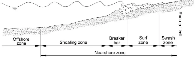
Figure 2-1: Simple example of a cross-shore profile + terminology

2.

Research background

2.1. Introduction

In this research several hydrodynamic and transport processes, which are of large importance, are described in this chapter. In the first paragraph a description of hydrodynamic aspects is given, followed by sediment transport aspects in the next paragraph. At the end of this chapter, it is described how the transport and hydrodynamic aspects influence sediment transport and thus also cross-shore morphology.

2.2. Hydrodynamic aspects 2.2.1. Wave propagation

Waves near the coast can be divided into three classes based on their wave period

(Dean & Dalrymple, 2002). The first class consist of wind waves and swell with typical

periods of 1-25 seconds and varying in wave height. These short waves travel in wave groups which propagate with the wave group velocity. In deep water the wave group velocity is equal to half the celerity of individual waves. Waves propagate into more shallow water slow down until their velocity is equal to the wave group velocity. The waves lengths get shorter, the waves change direction (refraction) towards the normal of the coast line, become higher (shoaling) and change in shape (non-linearity). Meanwhile, the waves loose energy smoothly due to dissipation by bed friction and in a short period of time by breaking in really shallow water.

A second class of waves is formed by “low-frequency waves” (infra-gravity waves). They are generated at open sea by group-behaviour of wind waves. Their periods range between 20-100 seconds. Low-frequency waves include both free and forced waves. In the surf zone low-frequency waves become free, because the wind waves that cause the forcing are decaying there. At the shore these long waves reflect and can even get trapped in the surf zone.

The third class of waves is formed by tidal waves. In the Netherlands the important tidal components are within the diurnal and semi-diurnal regime in which the most important constituent is the semi-diurnal lunar contribution (a period of 12 hours and 25 minutes). 2.2.2. Orbital motion

(18)

0 0.2 0.4 0.6 0.8 1

-1.5 -1 -0.5 0 0.5 1 1.5 t/T u (m /s ) (a)

0 0.2 0.4 0.6 0.8 1

[image:18.595.70.455.91.230.2]

-1.5 -1 -0.5 0 0.5 1 1.5 t/T u (m /s ) (b)

Figure 2-2: Free-stream velocity under skewed (a) and asymmetric (forward leaning) wave (b) compared to a sine wave.

0.5 0.55 0.6 0.65 0.7 0.75 0.8 0.85 0 0.2 0.4 0.6 0.8 1 1.2 1.4 R Sk (a)

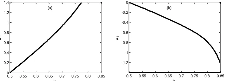
[image:18.595.75.452.576.711.2]

0.5 0.55 0.6 0.65 0.7 0.75 0.8 0.85 -1.2 -1 -0.8 -0.6 -0.4 -0.2 0  As (b)

Figure 2-3: Relation between the wave form parameters using the formula of Abreu et al. (2010, see par.4.4 and Appendix B): (a) skewness R and Sk for only skewed (non-asymmetric) waves; (b) asymmetry β and As for only asymmetric (non-skewed) waves.

Non-linearity consists of wave skewness (velocity skewness) and wave asymmetry (acceleration skewness), which are shown in Figure 2-2. Under skewed waves, the crest velocities become higher and the crest period shorter, while the trough velocities are lower and the trough period longer. Under asymmetric waves the acceleration and deceleration periods are not of equal length. There are two methods used to define the skewness and asymmetry of the orbital flow velocity. The first method is used in the SANTOSS formulations and states the skewness R and the asymmetry β as:

,max ,max

,max ,min .max ,min



 

 

w w

w w w w

u a

R

u u a a (2.2.1)

Where uw,max (uw,max) = the maximum velocity under the crest (trough) and aw,max (aw,min)

= the maximum acceleration (deceleration). For realistic conditions the values of both R and β range between 0.5 – 0.8, where both are 0.5 for sinusoidal waves. The other method is to use the time-averaged third power of the velocity scaled by the third power of the standard deviation to define the velocity skewness Sk (used by different authors like:

 

3 3 1.5 1.5 2 2   w w w w u u Sk As u u H (2.2.2)

(19)

conditions the range of Sk lies between 0  1.4 and the range of As between 0  -1.4 (Figure 2-2). Thus, both Sk and As are 0 for sinusoidal waves and for forward leaning wave asymmetry As becomes negative. Further in this report the parameters for skewness (R and Sk) and for asymmetry (β and As) are used several times, so these should be remembered very well and not be mixed up.

2.2.3. Currents

Waves induce a net transport of water towards the coast in the upper water layers, which induces set-up near the coast and currents. Different types of nearshore currents can be distinguished like wave-driven longshore currents, which are induced by waves approaching the coast under an angle (refraction of waves induce a long-shore momentum). Another type is a cross-shore current that is uniform in the longshore direction and which takes place in the lower layers (undertow). Especially under breaking waves this undertow can become high. The water that is transported towards the coast can also be returned by rip currents (non-uniform in longshore direction). The magnitude of these different currents lies in the order of 1 m/s.

2.2.4. Boundary layer flow

In shallow waters the near bed orbital velocity under waves is basically horizontal. At the bed the flow velocity is zero and due to viscosity the flow velocity above the bed is reduced due to the bed. The transition zone, between the bed and the point where the flow velocity is not anymore influence by the bed is called the boundary layer. Because most of the sediment transport takes place near the bed this process plays an important role in sediment transport (Dohmen-Janssen, 1999).

The thickness of the boundary layer depends on the Reynolds number (Re = Uw*Aw/ν)

and the relative roughness (ks/Aw) in which Uw is the orbital velocity amplitude, Aw is the

amplitude of the horizontal orbital displacement, ν is the kinematic viscosity and ks is

the bed roughness height. As a result the wave boundary layer for short waves is really small (order of centimetres) and for tidal waves the flow profile has almost a logarithmic profile like for currents.

Due to the lower velocities within the wave boundary layer, the flow in the boundary layer contains less inertia and reacts faster to varying pressure gradients. This is why the flow velocity in the boundary layer is ahead in phase to the free-stream velocity (for laminar flow 45º, for rough turbulent flow <45º).

A final important point about the hydrodynamics in the wave boundary layer is the streaming that is present. Despite of a mean velocity above the wave boundary layer there might be a different mean velocity present within the wave boundary layer. This may have two causes:

 Wave skewness causes a difference in generated turbulent energy between the two half-cycles, which leads to differences in the velocity profile in the wave boundary layer and a possible net streaming.

 The vertical and horizontal orbital velocities are not exactly 90° out of phase in the boundary layer as they would be in a frictionless flow (leads to an onshore-directed mean velocity close to the bed (Longuet-Higgins,

1953)).

2.3. Sediment transport aspects 2.3.1. Sediment properties

(20)

the grain sizes diameter is higher than 0.1 mm. If the sediment consists of a mixture of sand with different grain sizes, the grains of different sizes may influence each other. As said before, this research focuses on uniform sediment, so gradation effects are assumed to be low and thus not considered in this study.

2.3.2. Transport regimes in oscillatory flow

The different transport regimes in oscillatory flows are characterised by the bed forms and can be predicted based on the mobility number:





2 max

50 1

  

u

s gD (2.3.1)

In which umax = maximum orbital velocity, s = sediment specific gravity (2,65 for sand), g

= acceleration due to gravity and D50 = sediment grain size for which 50% of the

sediment sample is finer. The ripple regime is found for Ψ<190: bed forms are developed, ranging from small vortex ripples to large mega-ripples and dunes. At small vortex ripples twice every wave cycle a vortex is formed in the lee of the crest of the ripples, which results every time in sediment taken into suspension. Also 2D- and 3D ripples are observed which are linked to respectively large (<0.2 mm) and small grain sizes (>0.3 mm). The sheet-flow regime can be found for Ψ>300: at high orbital velocities the small ripples are washed out and the bed becomes plane. A thin layer with high sand concentrations is moving in a “sheet” over the bed. In the transition zone 190<Ψ<300 the bed is really sensitive.

Based on ripple dimension measurements under irregular waves it was recommended by O’Donoghue et al. (2006) to use the mean of the one tenth highest near bed velocities for the calculation of the mobility number. Furthermore, it must be mentioned that the dimensions of the bed forms cannot be predicted very well. Extensive measurements on bed forms under oscillatory flows have been taken place in oscillatory flow tunnels, but the influence of the realistic conditions (e.g. surface wave conditions and combination with currents) is not totally clear.

2.3.3. Bed shear stress and wave form effects

Sediment gets into motion due to bed shear stresses. The non-dimensional bed shear stress is defined by the Shields parameter ζ:





2 50 0.5

1

  



f u

s gD (2.3.2)

In which f = friction factor, which positive related to the orbital diameter and negatively related to the bed roughness height. This relation with the velocity above the bed would have explained the net bed-load transports under skewed waves. The roughness height depends largely on the sediment grain size and the ripple dimensions, but also a sheet flow (mobile-bed) increases the roughness. Overall, wave skewness is already taken into account quite well by different transport models. Due to the higher onshore velocities higher bed shear stresses are found under the crest and lower bed shear stresses under the trough.

(21)

on measurements in fixed bed flow tunnel experiments within the SANTOSS project

(Van der A, et al., 2008) and based on extensive model studies of sediment transport

processes under combined skewed and asymmetric waves using the PointSand Model (fully developed U-tube conditions) by Ruessink et al. (2009).

2.3.4. Unsteady effects in oscillatory flow

In steady flow the sand transport rate is proportional to a power (>1) of the near bed velocity. Many sediment transport models assume that the sediment transport in oscillatory flows also reacts instantaneously to the near bed orbital flow velocity or to the bed shear stress which is in some way related to the near bed flow velocity.

Unsteady effects are recognized when the phase lag between bed shear stress and concentration profiles (so no instantaneous reaction) leads to a change in sediment transport (Dibajnia & Watanabe, 1998; Dohmen-Janssen, 1999). Phase lag effects are especially of importance when the vertical sediment pick-up and settling processes take place at a time-scale of the same order as the wave period (in rippled-bed conditions or in sheet flow conditions for fine sediments, high orbital velocities and short wave periods). Due to phase lag effects net transport rates might be reduced or even change direction.

Ruessink et al. (2009) concluded also using their PSM modelling studies that phase lag effects are an essential mechanism for predicting transport rates. The wave-induced transport rates under velocity skewed waves reduce due to phase lag effects. They conclude that this reduction goes to zero, which means that the sediment transport is only determined by the current-related negative sediment transport.

2.3.5. Influence surface wave effects on sediment transport

Progressive surface waves induce Lagrangian and Eulerian effects (O'Donoghue &

Ribberink, 2007; Schretlen, et al., 2008), which might lead to a large difference in

transport rates compared to the same conditions in Oscillating Flow Tunnels, going up to a factor 2.5 (Dohmen-Janssen & Hanes, 2002). The Eulerian effects are already mentioned before (streaming due to skewness and Longuet-Higgins streaming) of which the Longuet-Higgins streaming is not present in an oscillatory flow tunnel, but also leads to an additional mean bed shear stress (Longuet-Higgins, 2005). The Lagrangian effect leads to extra onshore directed transport due to two processes that also count up to a certain amount for sediment particles:

 A fluid particle in a wave move with larger forward velocities at the top of its orbit compared to the backward velocities at the bottom.

 The fluid particles move with the wave during its forward motion and against it during its backward motion, and they thus experience a longer crest period and a shorter trough period.

2.4. Morphological aspects and modelling

Waves, current and sediment transport in coastal areas depend strongly on the bathymetry. Spatial gradients in sediment transport rates modify the bathymetry, which leads to feedback to the wave and current patterns and the resulting sediment transport. A strong feedback is visible in a coastal system and due to the ever changing wave conditions the system keeps trying to find a new equilibrium. Examples of changes are migration or deformation of sand dunes, trenches, and erosion/accretion of beaches. Especially in the nearshore zone of sandy beaches changes in morphology are clearly visible (e.g. on- or offshore migration of sand bars).

(22)

wateris about 1 m, peak wave period is about 6 s, the tidal range is 1.5-3.0 m, sediment grain sizes of about 300 μm and the near shore zone has a width of several hundreds of meters and a bottom slope of about 1:200). A large part of the Dutch coast is further characterized by 2 or 3 adjacent sand bars parallel to the shore line.

The generation and decay of a sandbar happens slowly over time and shows a cyclic cross-shore behaviour, arising near the shoreline and slowly (on average 0.01 m/day) moving through the surf zone and finally decaying in the outer nearshore zone at depths of 5-7 m (Grasmeijer, 2002). Superimposed on these long-term changes are weekly and monthly on- and offshore fluctuations (with the order of 1 m/day).

Morphological process models have problems to reproduce the natural behaviour of coasts on timescales of a few days to weeks and have shown high uncertainty on longer terms (Ruessink, et al., 2007). Most of these models predict the amount of beach erosion pretty well. Beach erosion, for example offshore migration of sand bars, takes place during storms when large waves break on the bar. The feedback between breaking waves, undertow, suspended sediment transport, and the sandbar are important here.

On the other hand, the models have trouble to predict the recovery of the beach profile under calm conditions (Ruessink, et al., 2007; Van Rijn, et al., submitted). Accretion, for example onshore bar migration, is predicted for energetic and (almost) non-breaking wave conditions (especially swell conditions). Important in accretive conditions is the feedback between near-bed wave skewness, bed-load transport, stokes drift, and the sandbar, with negligible to small influence of bound infra-gravity waves.

2.5. Conclusions

(23)

3.

Model descriptions

3.1. Introduction

This chapter gives a description of the three different models used in this research. First, a short description is given of the morphologic model UNIBEST-TC followed by a description of the two sand transport models TRANSPOR2004 (Van Rijn, 2007a,

2007b) and SANTOSS (Ribberink, et al., 2010). At the end of this chapter a previous

comparison between the performances of the two sand transport models is discussed, which focused on the prediction of transport rates measured during experiments.

3.2. UNIBEST-TC

UNIBEST-TC is the cross-shore sediment transport module of the program package UNIBEST, which stands for UNIform BEach Sediment Transport (Bosboom, et al., 2000). All modules of this package consider sediment transports along a sandy coast which locally may be considered uniform in alongshore direction. UNIBEST-TC (TC: Time-dependent Cross-shore) is designed to compute cross-shore sediment transports and the resulting profile changes along any coastal profile of arbitrary shape under the combined action of waves, longshore tidal currents and wind. The model allows for constant, periodic and time series of the hydrodynamic boundary conditions to be prescribed. The UNIBEST-TC software can be used for several coastal problems, e.g.:

 Dynamics of cross-shore profiles;

 Cross-shore development due to seasonal variations of the incident wave field;

 Bar generation and migration;

 To check the stability of beach nourishments;

 To estimate the impact of sand extraction on the cross-shore bottom profile development.

The UNIBEST-TC model is a parametric cross-shore profile-model, which is based on coupled, wave-averaged equations of hydrodynamics (waves and mean currents), sediment transport and bed level evolution. The formulations are divided over 5 modules: (1) the wave propagation module, (2) the mean current profile module, (3) the wave orbital velocity module, (4) bed load and suspended load transport module, and (5) bed level change module. For each predefined time step the modules are called in succession to calculate the hydrodynamic and transport rates over a whole profile after which the bed level changes define the new bathymetry, which is used as input for the next time step.

3.2.1. Wave propagation module

(24)

3.2.2. Mean current profile module

Based on the local wave forcing, mass flux, tide and wind forcing, a vertical distribution of the longshore and cross-shore velocities is calculated, taking into account the near-bed streaming. The vertical distribution of the flow velocities is determined with the Quasi-3D approach of Reniers et al. (2004). Based on the local wave forcing, the mass flux, tide and wind forcing, a vertical distribution of the longshore and cross-shore velocities is calculated. The near-bed streaming is included in the calculations. In this module the Eulerian current velocities are also adjusted to get the GLM velocities (including Stokes drift) using the method of Walstra et al. (2000).

3.2.3. Near bed orbital velocity module

The near bed velocity signal (ub(t)) is constructed to have the same characteristics of

short-wave velocity skewness, amplitude modulation (unl(t)), bound infragravity waves

(ubw(t)), and mean flow (umean(t)) as a natural random wave field. The near bed velocity

is the sum of these three components: ub(t) = unl(t) + ubw(t) + umean(t).

Several theories (Rienecker & Fenton, 1981; Isobe & Horikawa, 1982; Van Thiel de

Vries, 2009; Ruessink & Van Rijn, in preparation) are available to develop a short wave

(regular wave) velocity time series including skewness and asymmetry. These models consist of a combination of sines and cosines with certain amplitudes which represent the right wave shape (in more detail discussed in paragraph 4.3).

An amplitude modulation is taken place to include the effect of wave groups, with the focus on the preservation of velocity skewness. The bound long wave velocity is calculated using the method of Roelvink and Stive (Bosboom, et al., 2000) (In more detail discussed in paragraph 4.5).

3.2.4. Sediment transport module

The transport formulations for both bed load and suspended sediment load of Van Rijn

(2007a, 2007b) are already implemented including the Bagnold approach to account for

bed slope-induced transport (see paragraph 4.3 for further explanation of slope effect). Problems can be noticed with the wet-dry boundary. In UNIBEST-TC an approach is used in which the most landward wet computational grid point at each time step is taken as the grid point where the non-dimensional wave period (Tp/(gh)0.5) exceeds a certain

factor (TDRY = 20-40) for the first time. For the range of wave periods considered in the present erosion cases, this implies that no hydrodynamic and transport computations are carried out in depths less than about 0.1 m (small-scale) and 0.5 m(large-scale test) respectively. The sediment transport rate at the last wet grid point is translated into an offshore or onshore advection of the dry grid points by extrapolation over part of the dry beach and dune profile (horizontal extent of the extrapolation is based on local run-up.) 3.2.5. Bed level change module

At the end of each time step the bed levels are updated through:



b s w, s c,



b q q q

z

t x

  

 _

  (3.2.1)

3.3. Two practical sediment transport models

Because of their relative simplicity, practical sand transport models instead of process-based models, are used in practice for sediment transport predictions. Three classes of practical sand transport models can be distinguished:

(25)

 Quasi-steady models relate the instantaneous sediment transport rates to some power of the instantaneous near bed flow velocity or bed shear stress

(Ribberink, 1998; Nielsen, 2006).

 Semi-unsteady models account for unsteady (phase lag) effects without modelling the detailed time-dependent horizontal velocity and vertical concentration profiles (Dibajnia & Watanabe, 1998; Dohmen-Janssen, et al.,

2002).

The two transport models considered in this study (SANTOSS and TRANSPOR2004) are different concerning this subdivision and include or exclude several effects discussed in Chapter 2. Below, the transport models are shortly described after which a previous comparison between the two sediment models (Ribberink, et al., 2010; Wong, 2010) is shortly discussed. An extensive description of the two transport models can be found in Appendix A.5.

3.3.1. TRANSPOR2004 sand transport model

TRANSPOR2004 makes a division between bed-load transport and suspended-load transport. The bed load transport is modelled in a quasi-steady way (the bed load transport is instantaneously related to the bed shear stress), and the suspended load is based on a time-averaged approach. An improvement towards hydrodynamic and morphological modelling was the introduction of a bed roughness predictor within the TR2004 model, which predicts bed forms and the experienced roughness by the flow over the bed.

Bed roughness predictor

TR2004 distinguishes wave-related and related bed roughness. The current-related roughness (ks,c) is computed from the roughness heights induced by ripples

(ks,c,r), mega-ripples (ks,c,mr) and in case of estuaries or rivers also dunes (ks,c,d, not for

coastal waters). For coastal areas: ks,c = [ks,c,r2 + ks,c,mr2]0.5. The wave-related bed

roughness is only linked to the ripples due to the small length-scale of the orbital motion (ks,w = ks,c,r). The bed roughness induced by these bed forms is linked to the

non-dimensional mobility number ΨTR2004 based on both the depth-averaged current and the

orbital motion:









0.5

2 2

, 2004

50 1

R w R

TR

V U

s gD

  

 (3.3.1)

In which VR = the representative depth-averaged velocity based on the velocity in the

lowest computational layer (assuming logarithmic profile) and Uw,R = the representative

peak orbital velocity amplitude = (0.5Uw,on3 + 0.5Uw,off3)1/3. Mega-ripples are expected

for ΨTR2004< 550 leading to a roughness of the order of ks,w,mr=0.01hd, ripples are

highest for ΨTR2004< 50 (ks,c,r=150D50) and are degrading until ΨTR2004> 250 into the

sheet flow regime (ks,c,r = 20D50). The bed roughness is calculated together with the

current profile (iterative process) and is further used for the suspended load transport rates.

Bed-load transport

In TR2004 the bed-load transport rates (qb) for sand (d50>62μm) are instantaneously

(26)

and coastal flow conditions (1 dataset from one field site based on mega-ripple migration under waves+currents conditions).

 

0.5 ' ' , , , 0.3 50 * , 1 2

b wc b wc b cr

b s

w b cr

t t

q t  D D   

 

     

    

   

    (3.3.2)

In which η’b,cw = bed shear stress related to the free-stream velocity near the bed and

the grain friction coefficient = 0.5ρwf’cw(Uδ,cw)2, ρs = sediment density, ρw = water

density, and D* = the dimensionless particle size = D50[(s-1)g/ν2]1/3. Uδ,cw is the

instantaneous velocity due to currents and waves.

Three comments can be made on the bed load transport formulations in UNIBEST-TC:

 For the wave-induced orbital velocity the free-stream velocity is used. Van Rijn (Van Rijn, 2007a) states that the current velocity at the edge of the wave boundary layer together with an additional representative streaming velocity. In UNIBEST-TC a different approach is used for the superimposed current, because the quasi-3D approach (Reniers, et al., 2004) is used for the mean current profile module. The mean current profile already includes the near bed streaming. This is why the mean velocity in the lowest computational point is used as superimposed current velocity which is added to the orbital velocity time series.

 As suggested by Van Rijn (2007a) the influence of acceleration effects is included by replacing the orbital velocity component by a “sediment mobilising velocity” Uζ(t) according to the time domain filter method of

Nielsen and Callaghan (2003). This aspect was not yet implemented in the UNIBEST-TC version that was provided in this research and is included in the formulations.

 In UNIBEST-TC the phase lag effects on the bed load transport (recognized by Dohmen-Janssen (1999)) are not included, as recommended by Van Rijn (2007a).

Suspended-load transport

The suspended-load transport formulations in TR2004 are based on a time-averaged approach and divide the suspended-load into current-related transport and wave-related transport. The current-wave-related suspended-load transport is based on the time-averaged vertical distribution of the concentration and fluid velocities:





, 1     



h a s c s UCdz q p (3.3.3)

In which qs,c is the current-related suspended load transport (m2/s), U(z) is the local

time-averaged velocity at height z, C is the local time-averaged sediment concentration at height z (kg/m3), p is the porosity (=0.4) and ρs is the sediment density (kg/m3).

The wave-related suspended sediment transport is defined as the transport of the sediment particles by the oscillating fluid component and is based on the amount of sediment in the suspension layer above the bed and a velocity skewness factor.





4 4

, ,

, 3 3

, , 1

w c w t a

s w pl

s

w c w t

Cdz U U q f p U U        _ _      



(3.3.4) where the term [(Uw,c)4-(Uw,t)4]/ [(Uw,c)3+(Uw,t)3] = the velocity skewness factor. Uw,c and

Uw,t are the peak orbital velocities under respectively the crest and the trough. δ is the

(27)

In TR2004 the suspended sediment concentration profile over the whole depth is determined using a reference concentration close to the bed and an advection-diffusion equation for the distribution over the depth. In the advection-diffusion equation the fall velocity of suspended sediment and mixing coefficient due to waves and current play a vital role. The suspended transport rates and concentration profiles are extensively validated on river, tidal and coastal data (304 datasets from 9 rivers and tidal estuaries and 54 datasets from the Egmond beach along the coast of the Netherlands). The model is even validated on measurements under partial breaking waves.

The phase lag factor predicts the reduction in the wave-related suspended transport due to phase lag effect or even changes the transport into offshore direction and is computed using:





, ,

tanh 100 s w r 0.1

pl cr cr

s p

k

f P P P P

w T

 

  _  _   (3.3.5)

The phase lag factor is not standard implemented and is an extra feature that is mentioned by Van Rijn, Walstra et al. (2007) and which is added in the UNIBEST-TC formulations.

3.3.2. SANTOSS sand transport model

The other sand transport model is the SANTOSS model (Ribberink, et al., 2010) which is based on the semi-unsteady model concept of Dibajnia and Watanabe (1998). The concept uses a half-cycle approach (Figure 3-1): it divides a wave cycle into a crest period (onshore velocities) and a trough period (offshore velocities) and defines per half-cycle the entrained and transported sediment and the amount of sediment, which is not yet settled down at the end of the half-cycle and is mainly transported during the next half cycle. The total sediment transport in the wave boundary layer is calculated according to:

2 2

c c c t t t

b c cc tc t tt ct

p cu c p tu t

T T T T

 

   

  _   _  _   _

    (3.3.6)

In which Φb = the non-dimensional sediment transport = qb/[(s-1)gD503]0.5, s = relative

density = ρs/ρw and g = the gravitational acceleration. The concept divides a wave cycle

into two half-cycles (a crest and trough) and uses the representative shear stresses (ζc

and ζt, based on combination of orbital velocity and mean current, Figure 3-2), the

representative entrained loads (Ωc and Ωt) and the total (Tc and Tt) and acceleration

periods (Tcu and Ttu) per half cycle to calculate the sediment transport. A phase lag

approach defines which part of an entrained sediment load is also transported during the same half cycle (Ωcc and Ωtt) or during the next half-cycle (Ωct and Ωtc).

Several modifications have taken place compared to the original model concept of Dibajnia and Watanabe (1998):

 Ripple dimensions are based on the formulations of O’Donoghue et al. (2006) and depend only on the orbital flow velocities;

 The bed shear stress is used as driving parameter instead of the near-bed velocity;

 The influence of different wave shapes (velocity- and/or acceleration-skewed) is accounted for by including asymmetry effects in the friction factor

(Van der A, et al., 2008) and in the definition of the phase lag parameter.

 The effects of flow unsteadiness (phase-lags) are modelled in a modified way using a phase lag parameter based on the necessary time for the stirred sediment to fall back to the bed. The sheet flow layer or ripple height is used as reference height and the deceleration periods as critical time periods.

(28)

Figure 3-1: Velocity time series in wave direction. Tc and Tt are respectively the crest and trough periods, Tcu and Ttu are the crest and trough acceleration time lengths. The current shifts the time series up or down and affects both the maximum velocities and the periods (Ribberink, et al., 2010).

Figure 3-2: Illustration of wave and current velocity vectors u tw( ) and u . The vector uc is the resultant

velocity vector at maximum velocity under the crest of the wave (Ribberink, et al., 2010).

wave cycle but also influences the half cycle and acceleration periods and maximum velocities.

 Specific effects of progressive surface waves are included in the model:

o Additional bed shear stress in the direction of wave advance due to boundary layer streaming;

o Adaptation of half-cycle periods due to the Lagrangian effect and;

o Vertical orbital velocities which enhance/oppose the settling of sediment and thus decrease/increase phase lag effects.

The empirical formulations of the recognized processes are calibrated on extensive measurements of net transport rates in oscillatory flow tunnels (OFT’s) and wave flumes (e.g. GWK), where the processes related to surface waves were relatively excluded and included. In the oscillatory flow tunnel experiments also measurements in the ripple regime were used (more about the data set can be found in the next paragraph).

(29)

3.3.3. Performance transport models (previous research on comparison transport predictions with experiment data)

The SANTOSS formulations have been compared to the TR2004 formulations in a previous research (Ribberink, et al., 2010; Wong, 2010), which primarily focused on the reproduction of a large amount of detailed transport measurements under different conditions. In total 221 transport wave-dominated measurements from the SANTOSS database (Van der Werf, et al., 2009) were used, among which skewed waves, asymmetric waves, waves+currents and surface waves (flume tunnel experiments). Measurement in both sheet-flow and rippled-bed regimes were present and all cases are for non-breaking waves conditions. Detailed data about the near bed orbital velocities and the current velocities were used as input.

For the comparison measured near-bed orbital velocity time series and current velocities were used and applied to the total formulations of SANTOSS. The same input is used for the bed-load transport formulations of TR2004 (Van Rijn, 2007a) including the filter method of Nielsen and Callaghan (2003) and the near-bed streaming as proposed in Van Rijn (2007a).

Table 3-1 shows the different subsets together with the performance of the two transport formulations on transport rate predictions. The overall performance of the SANTOSS model is better; especially for velocity skewed waves, acceleration skewed (asymmetric) waves, and for the rippled-bed regime in general, the prediction of the SANTOSS model is much better. Interesting is that for the few (realistic) conditions (the surface waves) the two models show exactly the same performance.

A few discussion points towards this comparison are:

 The SANTOSS model is calibrated on the data sets that are used to compare the predictions of the models in contrast to the Van Rijn model, which can explain the differences in performance.

 Only the bed-load transport formulations of TR2004 are used for the comparison. This while especially in the ripple regime (high roughness) and in case of high orbital velocities also sediment gets into suspension (according to the formulations of Van Rijn (2007b)).

 Finally, the TR2004 formulations are especially designed to perform well in morphological models under all possible conditions (the models demand relative simple and especially robust formulations).

Table 3-1: Comparison of the performance of TR2004 and SANTOSS on large amount of sand transport measurements (Ribberink, et al., 2010; Wong, 2010)

Number of data

TR2004 (bed-load) SANTOSS

211 Factor 2 Factor 5 Factor 2 Factor 5

Overall performance 221 43% 64% 77% 93%

Data sub-set: type of bed-form

Sheet flow regime 155 54% 79% 83% 96%

Rippled-bed regime 56 13% 20% 61% 84%

Data sub-set: Type of flow

Velocity skewed waves (no currents) 94 27% 46% 69% 89%

Acceleration skewed waves (no currents) 53 38% 60% 79% 98%

Waves with currents 50 66% 90% 86% 92%

(30)

3.4. Conclusions

This chapter gave a description of the coastal modelling system UNIBEST-TC and the two transport models that are of interest in this study: TR2004 and SANTOSS. The two transport models are calibrated on partly the same experimental data. The TR2004 formulations are based on extensive experiment measurements, but are also verified on field data (good agreement with river, tidal and coastal flow conditions). The SANTOSS model is calibrated on a large amount of detailed tunnel and flume experiments for both the ripple and sheet flow regime, but no field data are used for calibration or validation. The two transport models use different concepts. The TR2004 formulations consist of three parts of which the bed roughness predictor has a direct interaction with the hydrodynamics in the model (influences the input). The bed-load is defined using a quasi-steady intra-wave approach, while the suspended load is defined in at time-averaged way using a suspended concentration and velocity profile. The suspended load consists of a wave-related (taking place in a small layer above the bed) and current-related suspended load (over the whole depth). Wave boundary layer streaming and acceleration effects are included in the bed load formulations, while phase lag effects can be included in the wave-related suspended load. The effects of wave asymmetry and phase lag effects were not yet implemented in the provided UNIBEST-TC version and are added for further analysis in this research.

The SANTOSS model is more process-based and includes all transport components in the wave boundary layer (which is in principal the bed load and wave-related suspended load). The half-cycle model concept also includes wave form effects, unsteady (phase lag) effects and the recognized surface wave effects, although their formulations are different compared to TR2004.

The previous comparison between the bed load formulations of TR2004 and the SANTOSS model showed that the SANTOSS model performs better on the prediction of the transport rates measured in different experiments. Some comments can be made on this comparison, especially about the data used for the comparison (SANTOSS model is calibrated on this data) and the comparison with only the bed load formulations of TR2004. A detailed comparison between the SANTOSS model and the total TR2004 formulations can give more insight in the model behaviour under changing conditions. Therefore, in Chapter 5 a comparison between the total transport rates predicted by the two models is executed.

(31)

4.

Implementation SANTOSS model in UNIBEST-TC

4.1. Introduction

This chapter gives an extensive review about the implementation of the SANTOSS transport formulations in the coastal modelling system UNIBEST-TC. Several issues are reviewed and choices made during the implementation are substantiated. In the first paragraph a few changes to the original SANTOSS transport formulations are mentioned. Next, some theories about slope effects are mentioned and how this is taken into account in the SANTOSS model (par. 4.3). Then, theories about the orbital flow velocity induced by short waves are explored (par. 4.3) followed by the influence of wave groups (par. 4.5) and how a superimposed current is included (par. 4.6). Finally, it is discussed how possible suspended load transport above the wave boundary layer is included (par. 4.7).

4.2. The SANTOSS sand transport code

The SANTOSS Matlab code (provided by Ribberink et al. (2010)) can make sediment transport predictions for different conditions: e.g. currents alone, oscillating horizontal motion (U-tube) with or without currents and surface waves with or without currents. Only the part for surface waves with superimposed currents has been copied and translated into FORTRAN 77 language (in which UNIBEST-TC is written), taking into account that the near-bed orbital motion can also become zero (for example at deeper water with small wave period).

First a stand-alone version of the SANTOSS code in FORTRAN was made to check whether the code has any errors. For all possible conditions the predictions made by the FORTRAN code has been compared to the Matlab code to check whether the model gives exactly the same results.

Some small changes to the SANTOSS code have been made, which were necessary before implementation of the code was possible, which are discussed in this paragraph.

Coordinate system

The coordinate systems used by the SANTOSS model and UNIBEST-TC are different. The sand transport model assumes waves propagate in x-direction with currents at angle θ counter-clockwise from this direction. In UNIBEST-TC the waves propagate at angle ζ counter-clockwise from the cross-shore (x-) direction, and the net current

 

,



v u v has a component in cross-shore and alongshore (y-) direction. Using the following formula solves the discrepancy:

 

atan

 v u  (4.2.1)

Furthermore, SANTOSS computes the net transport rates in the direction of wave propagation (q_{b wa}_, ) and normal to this direction (q_{b wa}_,_ ), which are related to the UNIBEST-TC coordinate system in the following way:

, , ,

cos sin

sin cos

 



 

 

b x b wa b wa

b y b wa b wa

q q q

q q q (4.2.2)

Definition of the half-cycle periods and the acceleration periods

(32)

parameter β is used to define the acceleration periods in case of asymmetric waves

(Malarkey, 2008).

Two problems arise considering the input delivered by UNIBEST-TC. The first issue is that when waves are both skewed and asymmetric, the method used in the Matlab code to define the periods based on R and β does not lead to exact results. Besides, UNIBEST-TC delivers a time series as input. Another issue is that UNIBEST-TC generates an orbital flow velocity time series of multiple waves, which can be of different shape and length in case of wave group simulation (see for more details par 4.5).

These issues resulted into the choice to write an extra function which extracts numerically from a time series of a wave train the zero-crossings, maxima and minima. From these data it defines for an arbitrary amount of half-cycles the half-cycle periods, the acceleration periods and the maximum flow velocities. In a later stage, the Shields stresses and the entrained loads are calculated per half-cycle. The phase lag effect is applied over the wave train in which a part of the entrained load of a half-cycle is given to the next half-cycle in the wave train (the last half-cycle gives to the first one).

Combination of high current with low oscillatory velocities

The proposed half-cycle approach for waves in combination with a current can lead to problems when the component of the current velocity in the direction of the wave propagation becomes too high compared to the orbital velocity. In this case one of the half-cycles (crest or trough) can get really small and eventually disappear, which brings problems to the phase lag factor. Especially when (a part of) the waves break, a strong current can be generated, which can induce this problem.

The actual problem lies in the model concept of SANTOSS. Entrained sediment can only be transported in the same half-cycle or in the next. It is not possible to transport sediment over several half-cycles, while this might be the case especially when one of the half-cycles becomes really small or when (small) sediment is entrained to high levels.

To avoid errors while running the model, the code is changed in such a way that if a cycle disappears, the load that is directed to this cycle from the previous half-cycle, is directed to the next half-cycle. So for example: when a crest disappears, the load that is coming from the previous trough should be directed to the next trough. This is a simple modification and it must be mentioned that (under phase lag dominated situations) this does not lead to a smooth transition zone in net transport rates around the point where a half-cycle disappears. On the other hand, these conditions are not common for coastal areas and in case of for example a high undertow due to breaking waves, the sediment transport is dominated by current-related suspended transport.

Redefinition of experienced periods (Lagrangian grain motion)

For surface waves conditions (realistic conditions) sediment grains move in the direction of wave propagation under the wave crest and against the wave under the wave trough (Lagrangian motion). In this way they experience a longer crest period Tc,sw (= Tc + ΔTc) and a shorter trough period Tt,,sw (= Tt – ΔTt ). The extension /

reduction of the half-cycle period depend on the ratio of the wave propagation velocity c and the horizontal grain displacement during the half wave-cycle (orbital diameter) dg

and can be written as:

 dg

T

c (4.2.3)

(33)

15th March 2011, final report 1 1 2 2 ˆ ˆ g g c t

d _c d _c

T T T T

c u  c u 

 

   

  _  _   _  _

    (4.2.4)

Where u = the representative orbital velocity amplitude and the reduction factor ζ = 0.55

= the ratio of the horizontal grain-velocity amplitude and the free-stream velocity amplitude u. Because of the numerical definition of an arbitrary amount of half-cycles with possibly different time lengths and an arbitrary superimposed current it is not recommended to use the total wave period in this approximation. It is better to replace the wave period in formula (4.2.4) with twice the measured half-cycle period:

1 1 , , 1 1 ˆ ˆ 2 2 g g

c c t t

w c w t

d c d c

T T T T

c u  c u 

 

   

  _  _   _  _

    (4.2.5)

This is physically more correct and it does not lead to extra problems with disappearing half-cycles as mentioned above. The factor δ might need to be recalibrated, but the difference in period change is not large.

Vertical flow velocity for ripple-cases

One discussion point considering the calibration of the SANTOSS model is the influence of the vertical velocity on the settling velocity of the suspended sediment. Vertical velocities affect therefore the phase lag parameter for both crest (lower phase lag parameter, less phase lag effect) and trough (larger phase lag parameter, more phase lag effect). The influence of vertical velocity is only calibrated for sheet flow conditions, because the full-scale surface wave experiments in flumes focused all on sheet flow transport. As a result the settling/fall velocity is therefore corrected with the maximum vertical velocity at 3 times the height of the sheet flow layer thickness above the bed (under the crest the fall velocity is enhanced due to downward flow velocity and under the trough the fall velocity is reduced).

For ripple conditions the influence of vertical velocities cannot be calibrated, but according to Ribberink et al. (2010) vertical velocities at the level of 3 times the ripple height should be chosen for ripple conditions.

4.3. Influence of bed-slopes on sediment transport

Most transport formulas are based on transport measurements for (nearly) horizontal beds. The bed slope may affect the transport rates in three ways:

 The bed slope influences the local near-