Application of Neuro-Genetic Algorithm to Determine
Reservoir Response in Different Hydrologic Adversaries
Mrinmoy MajuMdeR, Rabindra Nath BaRMaN, Pankaj Kr. Roy,
Bipal Kr. jaNa and asis MazuMdaR
School of Water Resources engineering, jadavpur university, Kolkata, India
Abstract: The hydrologic adversaries like high magnitude storms, extreme dryness, aridity, more than normal demand for water etc. often cause a huge stress on the storage structures such as reservoirs and check dams. This stress implies a lot of adverse effects on the adjacent population. One of the major causes of floods and droughts were due to the mis-management of stored water during hydrologic adversaries. The present study tries to estimate the distribution of the surplus water in the case of hydrologic adversaries. In this regard, two years of daily discharge data of one of the reservoirs, Panchet, of the river Damodar was randomly selected and grouped into six categories based on their magnitude. Three neural models were built. One out of the three was selected due to better performance validating criteria. The behaviour of the inputs in the case of hydrologic abnormality was configured with respect to the available historical records and applied to the selected model. The output would give the magnitude of surplus in the case of the pre-configured hydrologic adversaries. Ac-cording to the results, the Panchet reservoir could not mitigate the stress created due to the applied hydrologic adversaries. The study was conducted with a single reservoir and one major hydrologic pattern of the decade. A more detailed study with the help of this approach could further improve the model estimation.
Keywords: neuro-genetic models; reservoir response; hydrologic uncertainities; multireservoir river basin
The decision support system (DSS) of a reservoir controles the amount of water supplied to different sectors like industry, domestic sector, agriculture etc. The risk from such decisions becomes more pronounced during severe hydrologic conditions such as a high demand in dry conditions, a low demand in wet conditions, an abnormal inflow, an excessive evaporation due to extremely dry climate, etc. The reservoirs become highly stressed during such adverse conditions and the reservoir management can avoid or induce at that time severe damages. Coulibaly et al. (2005) sug-gested a combined model approach to improve the forecast of the reservoir inflow and found that different approaches will work better for differ-ent watersheds, lead times, and types of evdiffer-ents. This conclusion was supported by WMO (1992),
Singh (1995), Singh and Woolhiser (2002), etc. One day ahead stream-flow forecasting by multiple-layer perceptron (MLP) networks at a daily time step was studied for 47 watersheds by Anctil and Rat (2005). Karaboga et al. (2004) proposed a control method based on fuzzy logic for the real-time operation of spillway gates of a reservoir during any flood of any magnitude up to the probable maximum flood. Ahmed and Sarma (2005) determined the efficiency of neuro-modelling algorithms on generation of synthetic stream flow. Majumder et al. (2007) proposed the pattern for maximum water use for the River Damodar catchments with the help of back propa-gation neural networks.
of many large storage based systems. However, in the pre-British period in India, there were practi-cally no large reservoir projects. Even in the British period, a few storage structures were built only at the beginning of this century. Post-independence India, however, has seen more than 60% of ir-rigation budgets going for Major and Medium (M & M) projects. India, with a geographical area of 3.3 million square kilometers, experiences ex-tremes of climate. The annual average rainfall in the country is about 1170 mm, which is equivalent to nearly 4000 mm. India’s irrigated agriculture sector has been fundamental to India’s economic development and poverty alleviation. Some 28% of India’s Gross Domestic Product (GDP) and 67% of employment are based on agriculture. Agriculture is the primary source of livelihood in rural areas, which account for 75% of India’s population and 80% of its poor. And, in turn, irrigation is the base for about 56%, possibly more, of total agricultural output. The rapid expansion of irrigation and drainage infrastructure has been one of India’s major achievements (Lahiri-Dutt 2000).
The present study tries to estimate the impact of hydrologic adversaries on the selected reservoir operation. The reservoir surplus was used to show the impact on the reservoir operation. Reservoir inflow and outflow along with the water supplied in different sectors were treated as the input. The pattern was encoded in three neural models and these models were used to estimate the surplus for the conditions observed in the periods of hy-drological extremities.
Study area
In this context, in the present study was selected the Panchet reservoir of the river Damodar, a multi-reservoir network which is controlled by Damodar Valley Corporation (DVC). DVC was India’s first river development project and second large-scale river project of the last century after the Tennessee Valley Authority (TVA) in USA. The British administrator, W.W. Hunter, in his Statistical Account of Bengal described Damodar floods as “rainwater rushing off the hills through innumerable channels into the river bed with such great force and suddenness that the water rose to form a gigantic head wave of great breadth and sometimes rising up to 1.5 metres in height”. The uncontrolled part of the catchment, comprising about 3200 km2, extends from below Maithon
and Panchet dams to Durgapur Barrage for about 60 km had faced many high intensity storms and plays a major role in the agricultural develop-ment of the area. The construction of additional dams in the upper reaches (i.e. above Panchet and Mithon) contributes significantly to the runoff. The problem of the distribution of stored water is always pronounced in DVC catchment. When there is enough storage, the supplied water is adequate but in the case of adverse conditions, i.e. when the storage becomes too high or low, the distribution of the surplus water becomes the main cause of hydrologic devastations (Lahiri-Dutt 2000). A brief description of the DVC catchment is given next.
Description of the river basin
The Damodar river which lies between the lati-tudes 23°30'N and 24°19'N and longilati-tudes 85°31'E and 87°21'E, originates from the Palamu Hills of Chota Nagpur at an elevation of about 610 m above the mean sea level. It flows in south easterly direc-tion, entering the deltaic plains below Raniganj in Burdwan district of West Bengal, India. Near Burdwan, the river abruptly changes its course to southerly direction and joins the Hoogli river about 48 km below Kolkata. The slope of the river bed during the first 241 km is about 1.89 m/km. During the next 161 km it is about 0.57 m/km, fol-lowed by about 0.19 m/km in subsequent 145 km. The river is fed by six streams of which the princi-pal tributary, the Barakar, joins it where the river Damodar emerges from the Palamu Hills. The four main multipurpose reservoirs are located at Tilaiya, Konar, Maithon, Panchet, and Barrage at Durgapur was commissioned during 1953–1959. Another tributary, the Khudia, whose catchment is intercepted neither by Maithon nor Panchet reservoirs, joins the Damodar near its confluence with the Barakar. In the plains, the river splits into several channels and ultimately joins the rivers Roopnarayan & Hoogli. The total length of the river is about 541 km. The total catchment area of the river is 28 015 km2 of which 10 985 km2 lies under
Panchet (Konar – 997 km2, Tenughat – 4500 km2,
and Panchet 5488 km2) and 6293 km2 under Maithon
(Tilaiya – 984 km2, and Maithon – 5309 km2).
Climate of the river basin
Da-modar valley is 126 cm in Barakar, 127.2 cm in Damodar, and 132.9 cm in the lower valley. 82% of the mean annual rainfall occurs during the four monsoon months from June to September. The mean daily temperature varies from 40°C to below 20°C in winters. The rainfall in this area during the monsoon season is mainly due to the passage of depressions and low pressure over and near the area and the active monsoon conditions due to the accentuation of the seasonal trough.
Geo-morphology
The upper portion of the catchment consists of rough, hilly regions, whereas the lower portion is of flat deltaic plane, nature.
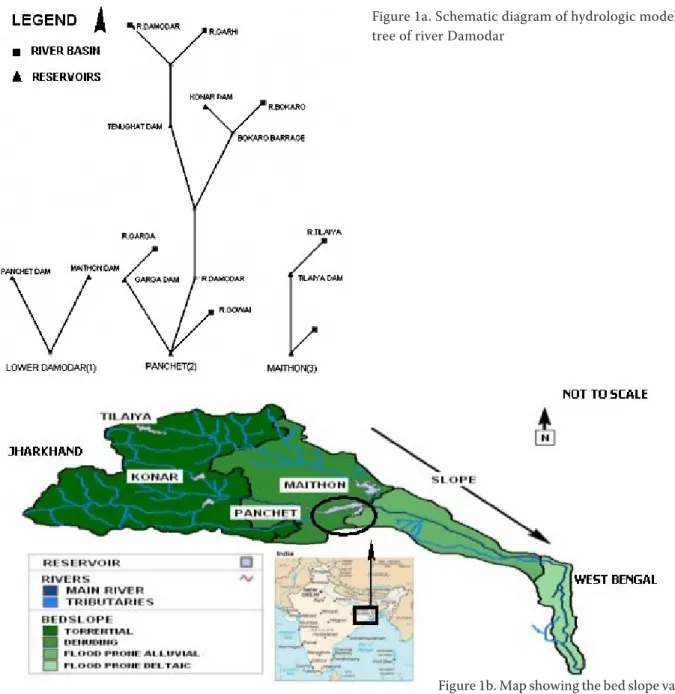
Figure 1a shows the network diagram of the River Damodar catchment in three parts. 1st part depicts the connectivity between the Panchet and Maithon sub-catchment with Durgapur Barrage. 2nd and 3rd part demonstrates the hydrologic modeling tree for the two (Panchet and Maithon) sub-catchment. In Figure 1b the Torrential bed slope represents deciduous forest, high slope and semi-pervious soil class. Denuding bed slope represents medium slope, non-arable land type with a soil class not conducive for agriculture. Flood-prone alluvial and deltaic bed slope represents flood prone regions of the basin with clayey and silty-loam soil.
The Panchet reservoir considered in the study falls within the Denuding (D) bed slope region.
Figure 1a. Schematic diagram of hydrologic modeling tree of river Damodar
Control structures
DVC has a network of four dams – Tilaiya and Maithon on the river Barakar, Panchet on the river Damodar, and Konar on the river Konar. Besides, Durgapur barrage and canal network, handed over to Government of West Bengal in 1964, remained a part of the total system of water management. Four multipurpose dams were constructed during the period of 1948 to 1959, namely Maithon, Panchet, Tilaiya, and Konar reservoirs. Out of these four reservoirs, the first three are used for hydropower generation. Konar is used only for agricultural purposes of the adjacent area. Though the water supplied for hydropower generation is allowed to return back to the reservoir, a small percentage of water gets diverted or evaporated. Panchet has a capability of 80 MW of power generation and a part of the supplied water is used up for this purpose (Roy et al. 2004).
Objective
The objective of the present study is to estimate the distribution of the surplus water in the case of various hydrologic adversaries. The study helps to identify whether or not the impact of the ad-versaries could be mitigated by a reservoir. In this regard, two years of daily discharge data of one of the reservoirs of the DVC system was randomly selected and grouped into six categories based on their magnitude of discharge. Three neural models were built. One of the three models was selected because it showed the most consistent validation performance. The behaviour of the inputs in the case of hydrologic abnormality was configured with respect to the available historical records (CWC 2005) and applied to the selected model. The output would give the magnitude of surplus in the case of the pre-configured hydrologic ad-versaries. According to the results, the Panchet reservoir would be in high stress when the applied hydrologic adversaries should happen in reality.
Data description
Daily reservoir discharge data, i.e. inflow, out-flow, reservoir storage, and water supply data, i.e. water used for irrigation, industry, and domestic use of Panchet reservoir for the year 1997–1998, were considered as the input and water surplus, calculated with the help of water supply dataset was considered for output. The water surplus of
the reservoir was calculated using the formula prescribed by Majumder et al. (2007).
The correlation coefficient of the output data series with the input data sets were –0.74, –0.76, –0.74, 0.04, 0.58, 0.47, and 0.04, respectively, for water used in domestic, industrial, and hydropower sectors; storage, inflow, and outflow. The mean values for the output and input data series were found to be equal to 49.44 and 1.54, 13.58, 26.34, 270.18, 14.74, 15.15, 142.48, respectively, for the surplus and water used in domestic, industrial, and hydropower sectors; storage, inflow, outflow, and water level. The output data series were found to be platykurtic (–1.54) and kurtosis of the input datasets were derived as 6.01, 0.80, –0.93, 683.95, 8.38, 21.32, and 683.95, respectively, for water used in domestic, industrial, and hydropower sectors; storage, inflow, outflow, and water level.
The variation of the output data series was 43.71 whereas that of the input data series were 1.74, 14.66, 28.01, 906.25, 24.48, 28.36, and 477.90, re-spectively, for water used in domestic, industrial, and hydropower sectors; storage, inflow, outflow, and water level data series.
According to the correlation measurements, the water use was found to be inversely related to the water surplus whereas the inflow, outflow, and level were found to be positively correlated with the output, although this relationship was not very pronounced. The central tendency measurements were found to be highly varied for the water level and storage. Other input data sets and the output showed moderate variations.
The output data series after clusterisation showed a standard deviation and mean value equal to 15.05 and 32.37 units, respectively.
MetHODOlOGy Artificial neural network
An artificial neural network (ANN) is a flexible mathematical structure that is capable of identify-ing complex nonlinear relationships between the input and output data sets. The ANN model of a physical system can be considered with n input neurons (x1, x2...xn), h hidden neurons (z1, z2....
zn), and m output neurons (y1, y2...yn). Let tj be the bias for neuron zj and fk for neuron yk. Let wij
be the weight of the connection from neuron xi
to zj and beta the weight of the connection zj to
natural genetic and natural selection. The basic elements of natural genetics – reproduction, cross-over, and mutation – are used in the genetic search procedure. A GA can be considered to consist of the following steps (Burn & Yulianti 2001): (1) Select an initial population of strings. (2) Evaluate the fitness of each string.
(3) Select strings from the current population to mate.
(4) Perform crossover (mating) for the selected strings.
(5) Perform mutation for selected string elements. (6) Repeat steps 2–5 for the required number of
generations.
Genetic algorithm is a robust method of searching the optimum solution to complex problems like the selection of optimal network topology where it is difficult or impossible to test for optimality. The basics of GA have already been discussed by many authors like Wang (1991), Wardlaw & Sharif (1999), Ahmed and Sarma (2005). Hence, the details of the basic procedures of GA are not focused on in the present literature.
Training phase
To encapsulate the desired input-output rela-tionship, the weights are adjusted and applied to the network until the desired error is achieved. This is called as “training the network”. There is innumerable number of “training the network” algorithms, among which back-propagation (ASCE 2000b) is mostly preferred. In the present study, Batch Back Propagation (BBP), Incremental Back Propagation (IBP), and Levenberg-Marquardt (LM), each of them derived from the basic back-propagation algorithms, are used as the training algorithm in this present study.
BBP is an advanced variant of Back Propagation where the network weights update takes place once per iteration.
IBP is a variation of the Back Propagation where the network weights are updated after presenting each case from the training subset, rather than once per iteration. This is an originally invented variant of back propagation and sometimes referred to as Standard Back Propagation.
LM (Kisi 2007) is an advanced non-linear op-timisation algorithm. It is the fastest algorithm available for multi-layer perceptrons. However, it has the following restrictions:
It can only be used on networks with a single output unit.
yk = ga (Σzibjk + fk) … (j = 1 – h) (1)
In which,
zj = fa (Σxiwij + tj) … (i = 1 – n) (2) where:
gA, fA – activation functions (Sudheer 2005)
The development of an artificial neural network, as prescribed by ASCE (2000a) follows the follow-ing basic rules,
(1) Information must be processed at many single elements called nodes.
(2) Signals are passed between nodes through con-nection links and each link has an associated weight that represents its connection strength. (3) Each of the nodes applies a non-linear
transfor-mation called activation function to its net input to determine its output signal.
The numbers of neurons contained in the input and output layers are determined by the number of input and output variables of a given system. The size or number of neurons of a hidden layer is an important consideration when solving the problems using multilayer feed-forward networks. If there are fewer neurons within the hidden layer, there may not be enough opportunity for the neural network to capture the intricate rela-tionships between the indicator parameters and computed output parameters. Too many hidden layer neurons not only require a large computa-tional time for accurate training, but may also result in overtraining. A neural network is said to be “over-trained” when the network focuses on the characteristics of the individual data points rather than just capturing the general patterns present in the entire training set. The network building procedure is divided into 3 phases which are described further.
Network building procedure Selection of network topology
It can only be used with small networks (a few hundred weights) because its memory requirements are proportional to the square of the number of weights in the network.
Testing phase
After training is completed, some portion of the available historical dataset is fed to the trained network and the known output is estimated out of them. The estimated values are compared with the target output to compute the mean square error (MSE). If the value of MSE is less than 1%, the network is said to be sufficiently trained and ready for the estimation. The dataset is also used for cross-validation to prevent over-training dur-ing the traindur-ing phase (Sudheer 2005).
In the present study, the IBP, BBP, and LM al-gorithms are used to train the model. The best model was selected with the help of the perfor-mance validation criteria as explained in the next section.
Evaluation of the network
The accuracy of the results obtained from the network is assessed by comparing its response with the validation set. The commonly used evalu-ation criteria include the correct classificevalu-ation rate (CCR), correlation coefficient (R) and Standard Deviation (SD) (Bhatt etal. 2007).
CCR = ((Tpc – opc)/Tpc) × 100 (3)
R = [Σ((Tp – Tm)(op – om))/(Σ(Tp – Tm)2 Σ(op – om)2)½] (4)
SD = Σ(Tn – Tn)2 (5) n
where:
Tpc – group of the actual dataset opc – estimated group
Tp – target group for the pth pattern op – estimated group for the pth pattern
Tm,om – mean target and estimated groups, respec-tively, and n is the total number of patterns.
CCR is used in the classification tasks as a quali-tative characteristic. This rate is calculated by di-viding the number of correctly recognised records by the total number of records. CCR is measured in relative units or in percents. R is the degree of correlation between two variables. In the present
study, the actual and predicted data series were grouped. That is why Spearman’s Formula for Rank Correlation (Das 1991) was used to measure the relationship between the two data series. SD is the measure of deviation of the estimated value from the target output. As both of the data series were in a composite condition, the SD for the present study is calculated with the help of the formula given next:
(6)
where:
σTp – denotes SD fT – group frequency
N – total number of data in the series
The same formula is calculated for op. (Das 1991) (Eq. (6)). The SD for the actual and predicted series is found out by dividing SD of the actual series and SD of the predicted series. A perfect match between the observed data and model simulations is obtained when SD approaches 0.0.
ReSUlt AND DISCUSSION Model development
Three neural models were developed from the reservoir dataset within the selected time scale, among which the model with the smallestt MSE, highest R, and minimum SD was selected for the simulation work.
The input and output parameters were taken as explained in the following paragraph.
The objective of the study was to estimate the impact of dry and wet hydrologic conditions on the Panchet reservoir. The surplus water of any reservoir represents the available water after fulfill-ing the necessary demands. The amount of water also determines the hydrologic stress of a reservoir. A high surplus implies that the reservoir is in an unstressed condition. The opposite reveals the stressfulness of the same. Hence, as the output it was taken the amount of water used in domestic, industrial, hydropower sectors with reservoir stor-age, inflow; outflow, and water level were taken as the input. Hydrological data set of two years was collected from the maintenance authority of the reservoir and daily data of all the parameters were fed into the neural models.
The time scale is one of the major constraints of any estimation problem. In the present study,
2 2
¸ ¸ ¹ · ¨ ¨ © §
¦
¦
N fT N
fT p p
Tp
V
1
n
1
n n
in the selected time span. The entire data set was ranked in an ascending way with respect to the magnitude and categorised with the help of the rules explained in the next paragraph. Neural network is a universal classifier (Hassoun 1995). It can estimate clustered dataset with more ef-the time scale was not ignored but hydrologic
conditions and reservoir response to such condi-tions were given more weightage. The response of the Panchet reservoir was observed for two consecutive years and its response was analysed for the hydrologic conditions that were prevalent
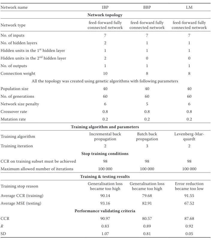
Table 1. Summary table showing optimum artificial neural network (ANN) model’s architecture and ANN internal parameters
Network name IBP BBP LM
Network topology
Network type connected networkfeed-forward fully connected networkfeed-forward fully connected networkfeed-forward fully
No. of inputs 7 7 7
No. of hidden layers 2 1 1
Hidden units in the 1st hidden layer 1 1 1
Hidden units in the 2nd hidden layer 2 0 0
No. of outputs 1 1 1
Connection weight 10 8 8
All the topology was created using genetic algorithms with following parameters
Population size 40 40 40
No. of generations 60 60 60
Network size penalty 6 5 6
Crossover rate 0.8 0.8 0.8
Mutation rate 0.2 0.2 0.2
training algorithm and parameters
Training algorithm Incremental back propagation propagationBatch back Levenberg-Mar-quardt
Training iteration 2 3 2
Stop training conditions
CCR on training subset must be achieved 98 98 98
Maximum allowed number of iterations 100 000 100 000 100 000
training & testing results
Training stop reason Generalisation loss became too high Generalisation loss became too high Error reduction became too low
Average CCR (training) 90.14 79.68 91.55
Average MSE (testing) 93.16 82.91 67.52
Performance validating criteria
CCR 90.97 80.57 87.68
R 0.83 0.89 0.92
SD 1.07 0.81 0.05
Fig.2.a
Ȭ3 Ȭ2 Ȭ1 0 1 2 3
1 2 3 4 5 6 7 8
Fig.2.b
Ȭ3 Ȭ2 Ȭ1 0 1 2 3
1 2 3 4 5 6 7 8
Fig.2.c
Ȭ3 Ȭ2 Ȭ1 0 1 2 3
1 2 3 4 5 6 7 8
Fig.2.d
Ȭ3 Ȭ2 Ȭ1 0 1 2 3
1 2 3 4 5 6 7 8
Fig.2.e
Ȭ3 Ȭ2 Ȭ1 0 1 2 3
1 2 3 4 5 6 7 8
Fig.2.f
Ȭ3 Ȭ2 Ȭ1 0 1 2 3
1 2 3 4 5 6 7 8
Fig.2.g
Ȭ3 Ȭ2 Ȭ1 0 1 2 3
1 2 3 4 5 6 7 8
Fig.2.h
Ȭ3 Ȭ2 Ȭ1 0 1 2 3
1 2 3 4 5 6 7 8
Figure 2. Figure showing the reservoir surplus for different hydrologic conditions as found from the historical data set
(A) low inflow in the reservoir (B) dry climatic condition
(C) low storage and high demand (D) low demand
ficiency than any other model. As every neural model follows a binary system of encoding, the accuracy of the neural model increases if clustered dataset is used.
As unstable dataset is defined such dataset which separates maximum or minimum from others. These datasets help to determine the threshholds of the entire data set. To be more precise, each peak and each trough borders the stability of the data set. And if the categorisation of the data set is done with respect to the stability of the param-eters, the output is said to be a more accurate representation of the problem (Parasuraman & Elshorbagy 2007).
The rules by which the dataset was classified are given next:
(1) If the rank of the data is below 5, then the data is clustered into group P (peak).
(2) If the rank of the data is below 15 but greater than 5, then the data is clustered into group MP (mid-peak).
(3) If the rank of the data is below 250 but greater than 15, then the data is clustered into group LP (low-peak).
Table 2. Table showing the values represented in Figure 2
Value in
the curve Category/Parameter X axis Parameter
1 reservoir level (input) 2 reservoir inflow (input) 3 reservoir outflow (input) 4 reservoir storage (input)
5 water used for hydropower( input) 6 water used for industrial sector (input) 7 water used for domestic sector (input) 8 reservoir surplus (output)
y axis category
3 P
2 MP
1 LP
–1 LT
–2 MT
–3 T
P – peak, MP – mid-peak; LP – low-peak; LT – low trough; MT – mid-trough; T - trough
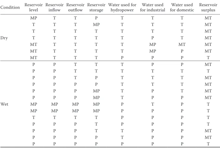
Table 3. Table showing reservoir surplus under dry and wet hydrologic adversaries
Condition Reservoir level Reservoir inflow Reservoir outflow Reservoir storage Water used for hydropower for industrialWater used for domesticWater used Reservoir surplus
Dry
MP T T P T T T MT
T T T MP T T T MT
T T T T T T T MT
T T T T T P T MT
MT T T T T MP MT MT
MT T T T T MP P MT
MT T T T P P P T
Wet
P P T T T P P MT
P P T T T T T T
P P T P T T T MT
P P P P T T T MT
P P P MP T P T MT
P P P MP T P P MT
MP MP MP MP P T P T
MP MP MP MP P P P T
T T T T P P P T
P P P T P P P T
P P P T T P P MT
P P P P T P P MT
P P P P P P P T
(4) If the rank of the data is below 500 but greater than 250, then the data is clustered into group LT (low trough).
(5) If the rank of the data is below 550 but greater than 500, then the data is clustered into group MT (mid-trough).
(6) If the rank of the data is greater than 550 then the data is clustered into group T (trough).
The minimum and maximum ranks were 1 and 731, respectively; as total 730 data were applied to the neural models to train the same.
68.18% of the clustered data set was used for training and 15.91% each of the same dataset were used for cross validation and testing purposes. Table 1 shows the MSE and absolute error after training and testing datasets. The model architec-ture and connection weight are also shown.
The network topology was selected the genetic algorithm and IBP, BP, and LM were used as the training algorithms to find the optimum result. The average CCR after training with LM algorithm was found to be 91.55% which is by 114.89% and 100.63% greater than BP and IBP networks, respec-tively. The average CCR after testing for LM was 67.52, i.e. 0.81 and 0.72 times the CCR achieved with IBP and BP, respectively.
The predicted results from LM achieved a CCR of 87.68% which was 1.08 times and 0.96 times the CCR found from BP and IBP networks. The CCR of IBP was greater than that of LM but IBP was found to be 110.84% less associated than LM which had 92% positive association with the target data series. LM had 5% deviation whereas IBP and BP had 107% and 81% deviation, respectively. The connection weight of LM was also 0.8 times smaller than that of IBP. According to the performance validation criteria and connection weight of the networks, LM was selected as the best model out of the three even if the CCR of IBP was greater than that of LM. As the connection weight is di-rectly related to the amount of data required for training that network, the requirement of heavier data is not conducive for the simulation.
The selected model was applied to estimate the surplus water of a reservoir with respect to dry and wet hydrologic adversaries. Figure 2 (a–h) depicts the surplus of the reservoir due to the reservoir inflow and outflow, water use, and reservoir level in dry and wet climatic conditions as found from the historical dataset. X axis denotes the input and output whereas y axis depicts the grouped data set. The table represents the input and output values.
The hydrologic adversaries were created by changing the input category. The adversaries were divided into two groups. The first group repre-sents the stresses in a dry hydrologic conditions and next group represents the stresses that comes with wet hydrologic conditions. Incase of both of the adversaries the reservoir surplus becomes very low or low. That concludes that the reservoir will be in a huge negative stress in the case of various hydrologic adversaries (Table 3). This was eminent in the result given in the last row of the table where all the inputs were grouped into the maximum but still the surplus shows a low value. The ob-servations of the results also conclude that there is some specific impact of water use on surplus which is natural. This help to verify the practicality of the model. Even when the reservoir inflow and outflow were high and the demands were low, the surplus still falls into the lowest group. Thus from the results it could be clearly concluded that the reservoir would be in stress for both dry and wet hydrologic adversaries.
CONClUSION
Corresponding author:
Mrinmoy Majumder, ME, Senior Research Fellow, School of Water Resources Engineering, Jadavpur University, 700032 Kolkata, India
e-mail: [email protected]
The present study can be improved if separated models are developed for separate seasons. The same can be done for different types of storms observed in the basin.
References
Ahmed J.A., Sarma A.K. (2005): Genetic algorithm for optimal operating policy of a multipurpose reser-voir. Journal of Water Resources Management, 19: 145–161.
Anctl F., Rat A. (2005): Evaluation of neural network stream flow forecasting on 47 watersheds.Journal of Hydrologic Engineering, 10: 85–88.
ASCE (2000a): Task committee on application of arti-ficial neural networks in hydrology. Artiarti-ficial neural networks in hydrology I: Preliminary concepts. Journal of Hydrologic Engineering, 5: 115–123.
ASCE (2000b): Task committee on application of arti-ficial neural networks in hydrology. Artiarti-ficial neural networks in hydrology II: Hydrologic applications. Journal of Hydrologic Engineering, 5: 124–132. Bhatt V.K., Bhattacharya P., Tiwari A.K. (2007):
Application of artificial neural network in estimation of rainfall erosivity. Hydrology Journal, 1–2: 30–39. Burn D.H., Yulianti J.S. (2001): Waste-load allocation
using genetic algorithms. Journal of Water Resources Planning and Management, 127: 121–129 (Retrieved from link.aip.org on January, 2008).
Central Water Commission (CWC) (2005): Databook of Reservoir Operation Daily Data. Damodar Valley Corporation, Kolkata.
Coulibaly P., Haché M., FortinV., Bobée B. (2005): Improving daily reservoir inflow forecasts with model combination. Journal of Hydrologic Engineering, 10: 91–99.
Das N.G. (1991): Statistical Methods. Part 1, M. Das & Co., Kolkata, 226–231.
Hassoun M.H. (1995): Fundamentals of Artificial Neural Networks. The MIT Press, New York, 1–2.
Karaboga D., Bagis A., Haktanir T. (2004): Fuzzy logic based operation of spillway gates of reservoirs during floods.Journal of Hydrologic Engineering, 9: 544–549.
Kisi Ö. (2007): Streamflow forecasting using different artificial neural network algorithms. Journal of Hy-drologic Engineering, 12: 532–539.
Lahiri-Dutt K. (2000): State and the Community in Water Management Case of the Damodar Valley Cor-poration, India. Report on Resource Management in Asia Pacific Program. In: Proc.Water Environment Partnership in Asia (WEPA). WEPA, Manilla. Majumder M., Roy P.K., Mazumdar A. (2007):
Opti-mization of the water use in the river Damodar in West Bengal in India: An integrated multi-reservoir system with the help of artificial neural network. Journal of Engineering, Computing and Architecture. 1: Article No. 1192.
Parasuraman K., Elshorbagy A. (2007): Cluster-based hydrologic prediction using genetic algorithm-trained neural networks. Journal of Hydrologic Engineering, 12: 52–62.
Roy P.K., Roy D., Mazumdar A. (2004): An impact assessment of climate change and water resources availability of Damodar river basin. Hydrology Journal, 27: 53–70.
Singh V.P. (1995): Computer Models of Watershed Hydrology. Water Resource Publications, Highlands Ranch.
Singh V.P., Woolhiser D.A. (2002): Mathematical mod-eling of watershed hydrology. Journal of Hydrologic Engineering, 7: 270–292.
Sudheer K.P. (2005): Knowledge extraction from trained neural network river flow models. Journal of Hydrologic Engineering, 10: 264–269.
Wang Q.J. (1991): The genetic algorithm and its applica-tion to calibrating conceptual rainfall-runoff models. Water Resources Research, 27: 2467–2471.
Wardlaw R., Sharif M. (1999): Evaluation of genetic algorithms for optimal reservoir system operation. Journal of Water Resources Planning and Manage-ment, 125: 25–33.
World Meteorological Organization (WMO) (1992): Simulated real time inter-comparison of hydrological models, Operational Hydrology Rep., 38, WMO No. 779, Geneva.