for Syntax-Based Machine Translation
Wei Wang
∗Language Weaver, Inc.
Jonathan May
∗∗USC/Information Sciences Institute
Kevin Knight
†USC/Information Sciences Institute
Daniel Marcu
‡ Language Weaver, Inc.This article shows that the structure of bilingual material from standard parsing and alignment tools is not optimal for training syntax-based statistical machine translation (SMT) systems. We present three modifications to the MT training data to improve the accuracy of a state-of-the-art syntax MT system:re-structuring changes the syntactic structure of training parse trees to enable reuse of substructures; re-labeling alters bracket labels to enrich rule application context; and re-aligning unifies word alignment across sentences to remove bad word alignments and refine good ones. Better structures, labels, and word alignments are learned by the EM algorithm. We show that each individual technique leads to improvement as measured by BLEU, and we also show that the greatest improvement is achieved by combining them. We report an overall 1.48 BLEU improvement on the NIST08 evaluation set over a strong baseline in Chinese/English translation.
1. Background
Syntactic methods have recently proven useful in statistical machine translation (SMT). In this article, we explore different ways of exploiting the structure of bilingual material for syntax-based SMT. In particular, we ask what kinds of tree structures, tree labels, and word alignments are best suited for improving end-to-end translation accuracy. We begin with structures from standard parsing and alignment tools, then use the EM algorithm to revise these structures in light of the translation task. We report an overall +1.48 BLEU improvement on a standard Chinese-to-English test.
∗6060 Center Drive, Suite 150, Los Angeles, CA, 90045, USA. E-mail: [email protected]. ∗∗4676 Admiralty Way, Marina del Rey, CA, 90292, USA. E-mail: [email protected].
†4676 Admiralty Way, Marina del Rey, CA, 90292, USA. E-mail: [email protected].
‡6060 Center Drive, Suite 150, Los Angeles, CA, 90045, USA. E-mail: [email protected].
We carry out our experiments in the context of a string-to-tree translation system. This system accepts a Chinese string as input, and it searches through a multiplicity of English tree outputs, seeking the one with the highest score. The string-to-tree frame-work is motivated by a desire to improve target-language grammaticality. For example, it is common for string-based MT systems to output sentences with no verb. By contrast, the string-to-tree framework forces the output to respect syntactic requirements—for example, if the output is a syntactic tree whose root is S (sentence), then the S will gen-erally have a child of type VP (verb phrase), which will in turn contain a verb. Another motivation is better treatment of function words. Often, these words are not literally translated (either by themselves or as part of a phrase), but rather they control what happens in the translation, as with case-marking particles or passive-voice particles. Finally, much of the re-ordering we find in translation is syntactically motivated, and this can be captured explicitly with syntax-based translation rules. Tree-to-tree systems are also promising, but in this work we concentrate only on target-language syntax. The target-language generation problem presents a difficult challenge, whereas the source sentence is fixed and usually already grammatical.
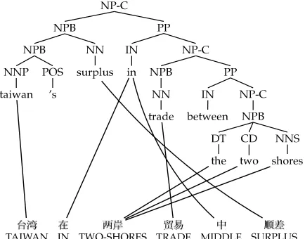
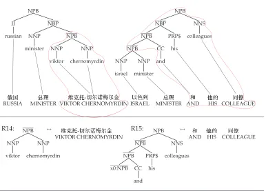
To prepare training data for such a system, we begin with a bilingual text that has been automatically processed into segment pairs. We require that the segments be single sentences on the English side, whereas the corresponding Chinese segments may be sentences, sentence fragments, or multiple sentences. We then parse the English side of the bilingual text using a re-implementation of the Collins (1997) parsing model, which we train on the Penn English Treebank (Marcus, Santorini, and Marcinkiewicz 1993). Finally, we word-align the segment pairs according to IBM Model 4 (Brown et al. 1993). Figure 1 shows a sample (tree, string, alignment) triple.
We build two generative statistical models from this data. First, we construct a smoothed n-gram language model (Kneser and Ney 1995; Stolcke 2002) out of the English side of the bilingual data. This model assigns a probability P(e) to any candidate translation, rewarding translations whose subsequences have been observed frequently in the training data.
[image:2.486.50.267.461.631.2]Second, we build a syntax-based translation model that we can use to produce candidate English trees from Chinese strings. Following previous work in noisy-channel
Figure 1
SMT (Brown et al. 1993), our model operates in the English-to-Chinese direction— we envision a generative top–down process by which an English tree is gradually transformed (by probabilistic rules) into an observed Chinese string. We represent a collection of such rules as a tree transducer (Knight and Graehl 2005). In order to construct this transducer from parsed and word-aligned data, we use the GHKM rule extraction algorithm of Galley et al. (2004). This algorithm computes the unique set of
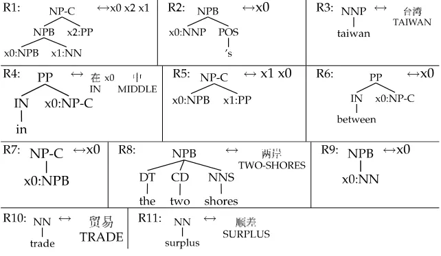
minimal rulesneeded to explain any sentence pair in the data. Figure 2 shows all the minimal rules extracted from the example (tree, string, alignment) triple in Figure 1. Note that rules specify rotation (e.g., R1, R5), direct translation (R3, R10), insertion and deletion (R2, R4), and tree traversal (R9, R7). The extracted rules for a given example form aderivation tree.
We collect all rules over the entire bilingual corpus, and we normalize rule counts in this way: P(rule)= count(countLHS-(ruleroot)(rule)). When we apply these probabilities to derive an English sentenceeand a corresponding Chinese sentencec, we wind upcomputing the joint probability P(e,c). We smooth the rule counts with Good–Turing smoothing (Good 1953).
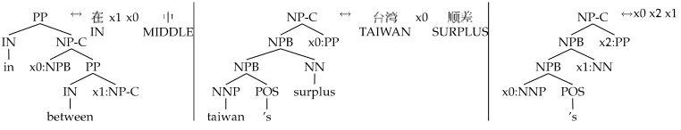
This extraction method assigns each unaligned Chinese word to a default rule in the derivation tree. We next follow Galley et al. (2006) in allowing unaligned Chinese words to participate in multiple translation rules. In this case, we obtain a derivation forestof minimal rules. Galley et al. show how to use EM to count rules over deriva-tion forests and obtain Viterbi derivaderiva-tion trees of minimal rules. We also follow Galley et al. in collectingcomposed rules, namely, compositions of minimal rules. These larger rules have been shown to substantially improve translation accuracy (Galley et al. 2006; DeNeefe et al. 2007). Figure 3 shows some of the additional rules.
[image:3.486.54.375.450.637.2]With these models, we can decode a new Chinese sentence by enumerating and scoring all of the English trees that can be derived from it by rule. The score is a weighted product of P(e) and P(e,c). To search efficiently, we employ the CKY dynamic-programming parsing algorithm (Yamada and Knight 2002; Galley et al. 2006). This algorithm builds English trees on topof Chinese spans. In each cell of the CKY matrix, we store the non-terminal symbol at the root of the English tree being built up. We also
Figure 2
Figure 3
Additional rules extracted from the learning case in Figure 1.
store English words that appear at the left and right corners of the tree, as these are needed for computing the P(e) score when cells are combined. For CKY to work, all transducer rules must be broken down, or binarized, into rules that contain at most two variables—more efficient search can be gained if this binarization produces rules that can be incrementally scored by the language model (Melamed, Satta, and Wellington 2004; Zhang et al. 2006). Finally, we employ cube pruning (Chiang 2007) for further efficiency in the search.
When scoring translation candidates, we add several smaller models. One model rewards longer translation candidates, off-setting the language model’s desire for short output. Other models punish rules that drop Chinese content words or introduce spurious English content words. We also include lexical smoothing models (Gale and Sampson 1996; Good 1953) to help distinguish good count rules from bad low-count rules. The final score of a translation candidate is a weighted linear combination of log P(e), log P(e,c), and the scores from these additional smaller models. We obtain weights through minimum error-rate training (Och 2003).
The system thus constructed performs fairly well at Chinese-to-English translation, as reflected in the NIST06 common evaluation of machine translation quality.1
However, it would be surprising if the parse structures and word alignments in our bilingual data were somehow perfectly suited to syntax-based SMT—we have so far used out-of-the-box tools like IBM Model 4 and a Treebank-trained parser. Huang and Knight (2006) already investigated whether different syntactic labels would be more appropriate for SMT, though their study was carried out on a weak baseline translation system. In this article, we take a broad view and investigate how changes to syntactic structures, syntactic labels, and word alignments can lead to substantial improvements in translation quality on topof a strong baseline. We design our methods around problems that arise in MT data whose parses and alignments use some Penn Treebank-style annotations. We believe that some of the techniques will apply to other annotation schemes, but conclusions here are limited to Penn Treebank-style trees.
The rest of this article is structured as follows. Section 2 describes the corpora and model configurations used in our experiments. In each of the next three sections we present a technique for modifying the training data to improve syntax MT accuracy: tree re-structuring in Section 3, tree re-labeling in Section 4, and re-aligning in Section 5. In each of these three sections, we also present experiment results to show the impact of each individual technique on end-to-end MT accuracy. Section 6 shows the improve-ment made by combining all three techniques. We conclude in Section 7.
2. Corpora for Experiments
For our experiments, we use a 245 million word Chinese/English bitext, available from LDC. A re-implementation of the Collins (1997) parser runs on the English half of the bitext to produce parse trees, and GIZA runs on the entire bitext to produce M4 word alignments. We extract a subset of 36 million words from the entire bitext, by selecting only sentences in the mainland news domain. We extract translation rules from these selected 36 million words. Experiments show that our Chinese/English syntax MT systems built from this selected bitext give as high BLEU scores as from the entire bitext. Our development set consists of 1,453 lines and is extracted from the NIST02– NIST05 evaluation sets, for tuning of feature weights. The development set is from the newswire domain, and we chose it to represent a wide period of time rather than a single year. We use the NIST08 evaluation set as our test set. Because the NIST08 evaluation set is a mix of newswire text and Web text, we also report the BLEU scores on the newswire portion.
We use two 5-gram language models. One is trained on the English half of the bitext. The other is trained on one billion words of monolingual data. Kneser–Ney smoothing (Kneser and Ney 1995) is applied to both language models. Language models are represented using randomized data structures similar to those of Talbot and Osborne (2007) in decoding for efficient RAM usage.
To test the significance of improvements over the baseline, we compute paired boot-strap p-values (Koehn 2004) for BLEU between the baseline system and each improved system.
3. Re-structuring Trees for Training
Our translation system is trained on Chinese/English data, where the English side has been automatically parsed into Penn Treebank-style trees. One striking fact about these trees is that they contain many flat structures. For example, base noun phrases frequently have five or more direct children. It is well known in monolingual parsing research that these flat structures cause problems. Although thousands of rewrite rules can be learned from the Penn Treebank, these rules still do not cover the new rewrites observed in held-out test data. For this reason, and to extract more general knowl-edge, many monolingual parsing models aremarkovizedso that they can produce flat structures incrementally and horizontally (Collins 1997; Charniak 2000). Other parsing systems binarize the training trees in a pre-processing step, then learn to model the binarized corpus (Petrov et al. 2006); after parsing, their results are flattened back in a post-processing step. In addition, Johnson (1998b) shows that different types of tree structuring (e.g., the Chomsky adjunction representation vs. the Penn Treebank II representation) can have a large effect on the parsing performance of a PCFG estimated from these trees.
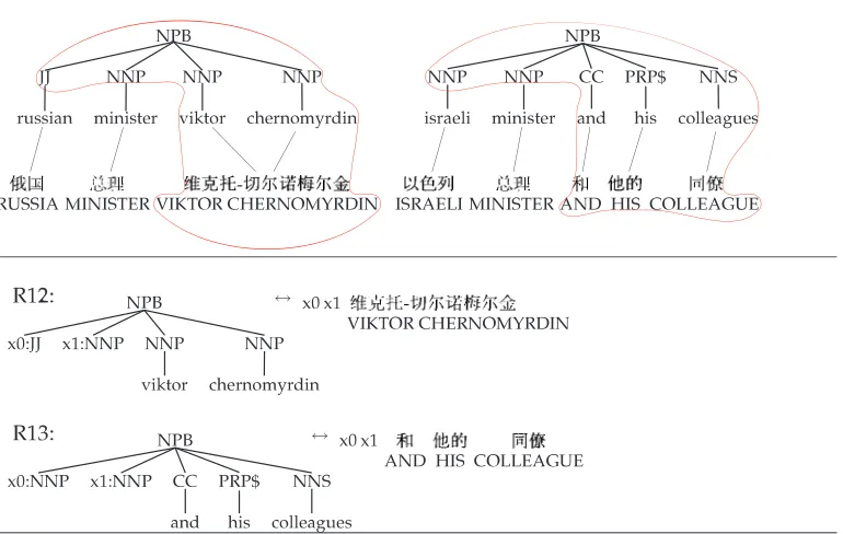
We find that flat structures are also problematic for syntax-based machine transla-tion. The rules we learn from tree/string/alignment triples often lack sufficient gener-alization power. For example, consider the training samples in Figure 4. We should be able to learn enough from these two samples to translate the new phrase
...WWW-###LLL
Z Z Z
ÆÆÆ{{{ 333äää
VIKTOR CHERNOMYRDIN AND HIS COLLEAGUE
Figure 4
Learning translation rules from flat English structures.
However, the learned rules R12 and R13 do not fit together nicely. R12 can translate
...WWW-###LLL into an English base noun phrase (NPB) that includes viktor
chernomyrdin, but only if it is preceded by words that translate into an English JJ and an English NNP. Likewise, R13 can translateZZZ ÆÆÆ{{{ 333äääinto an NPB that includes
and his colleagues, but only if preceded by two NNPs. Both rules want to create an NPB, and neither can supply the other with what it needs.
If we re-structure the training trees as shown in Figure 5, we get much better behavior. Now rule R14 translates...WWW-###LLLinto a free-standing NPB. This
gives rule R15 the ability to translateZZZ ÆÆÆ{{{ 333äää, because it finds the necessary
NPB to its left.
Here, we are re-structuring the trees in our MT training data bybinarizingthem. This allows us to extract better translation rules, though of course an extracted rule may have more than two variables. Whether the rules themselves should be binarized is a separate question, addressed in Melamed, Satta, and Wellington (2004) and Zhang et al. (2006). One can decide to re-structure training data trees, binarize translation rules, or do both, or do neither. Here we focus on English tree re-structuring.
Figure 5
Learning translation rules from binarized English structures.
3.1 Some Concepts
We now explain some concepts to facilitate the descriptions of the re-structuring meth-ods. We train our translation model on alignment graphs (Galley et al. 2004). An alignment graph is a tuple of a source-language sentencef, a target-language parse tree that yields eand translates from f, and the word alignmentsa betweene andf. The graphs in Figures 1, 4, and 5 are examples of alignment graphs.
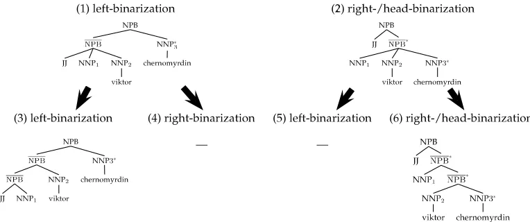
In the alignment graph, a node in the parse tree is calledadmissibleif rules can be extracted from it. We can extract rules from a node if and only if the yield of the tree node is consistent with the word alignments—thefstring covered by the node is contiguous but not empty, and the f string does not align to anye string that is not covered by the node. An admissible tree node is one where rules overlap. Figure 6 shows different binarizations of the left tree in Figure 4. In this figure, the NPB node in tree (1) is not admissible because thefstring, V-C, that the node covers also aligns to NNP3, which is not covered by the NPB. Node NPB in tree (2), on the other hand, is admissible.
A set of sibling tree nodes is called factorizable if we can form an admissible new node dominating them. In Figure 6, sibling nodes NNP1, NNP2, and NNP3 are factorizable because we can factorize them out and form a new node NPB, resulting in tree (2). Sibling tree nodes JJ, NNP1, and NNP2 are not factorizable. Not all sibling nodes are factorizable, so not all sub-phrases can be acquired and syntactified. Our main purpose is to re-structure parse trees by factorization such that syntactified sub-phrases can be employed in translation.
Figure 6
Left, right, and head binarizations on the left tree in Figure 4. Tree leaves of nodes JJ and NNP1 are omitted for convenience. Heads are marked with∗. New nonterminals introduced by binarization are denoted by X-bars.
3.2 Binarizing Syntax Trees
We re-structure parse trees by binarizing the trees. We are going to binarize a tree node
nthat dominatesrchildrenn1, ...,nr. Binarization is performed by introducing new tree nodes to dominate a subset of the children nodes. We allow ourselves to form only one new node at a time to avoid over-generalization. Because labeling is not the concern of this section, we re-label the newly formed nodes asn.
3.2.1 Simple Binarization Methods.Theleft binarizationof noden(e.g., the NPB in tree (1) of Figure 6) factorizes the leftmostr−1 children by forming a new noden(i.e., the NPB in tree (1)) to dominate them, leaving the last childnruntouched; and then makes
the new nodenthe left child ofn. The method then recursively left-binarizes the newly formed nodenuntil two leaves are reached. We left-binarize the left tree in Figure 4 into Figure 6 (1).
Theright binarizationof nodenfactorizes the rightmostr−1 children by forming a new node n (i.e., the NPB in tree (2)) to dominate them, leaving the first childn1
untouched; and then makes the new node n the right child of n. The method then recursively right-binarizes the newly formed node n. For instance, we right-binarize the left tree in Figure 4 into Figure 6 (2) and then into Figure 6 (6).
The head binarization of node n left-binarizes n if the head is the first child; otherwise, it right-binarizes n. We prefer right-binarization to left-binarization when both are applicable under the head restriction because our initial motivation was to generalize the NPB-rooted translation rules. As we show in experiments, binarization of other types of phrases contributes to translation accuracy as well.
Figure 7
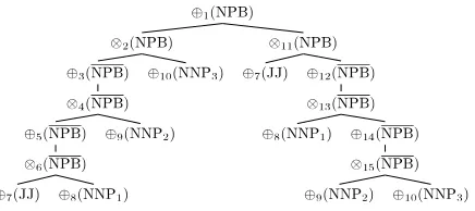
Packed forest obtained by packing trees (3) and (6) in Figure 6.
3.2.2 Parallel Binarization.Simple binarizations transform a parse tree into another single parse tree. Parallel binarization transforms a parse tree into a binarization forest, packed to enable dynamic programming when we extract translation rules from it.
Borrowing terms from parsing semirings (Goodman 1999), a packed forest is com-posed of additive forest nodes (⊕-nodes) and multiplicative forest nodes (⊗-nodes). In the binarization forest, a⊗-node corresponds to a tree node in the unbinarized tree or a new tree node introduced during tree binarization; and this⊗-node composes several ⊕-nodes, forming a one-level substructure that is observed in the unbinarized tree or in one of its binarized tree. A⊕-node corresponds to alternative ways of binarizing the same tree node and it contains one or more⊗-nodes. The same⊕-node can appear in more than one place in the packed forest, enabling sharing. Figure 7 shows a packed forest obtained by packing trees (3) and (6) in Figure 6 via the following tree parallel binarization algorithm.
We use a memoization procedure to recursively parallel-binarize a parse tree. To parallel-binarize a tree nodenthat has childrenn1,...,nr, we employ the following steps:
r
Ifr≤2, parallel-binarize tree nodesn1, ...,nr, producing binarization⊕-nodes⊕(n1), ...,⊕(nr), respectively. Construct node⊗(n) as the parent of⊕(n1),...,⊕(nr). Construct an additive node⊕(n) as the parent of⊗(n). Otherwise, execute the following steps.
r
Right-binarizen, if any contiguous2subset of childrenn2,...,nrisfactorizable, by introducing an intermediate tree node labeled asn. We recursively parallel-binarizento generate a binarization forest node⊕(n). We also recursively parallel-binarizen1, forming a binarization forest node⊕(n1). We form a multiplicative forest node⊗Ras the parent of
⊕(n1) and⊕(n).
r
Left-binarizenif any contiguous subset ofn1,...,nr−1is factorizable and if this subset containsn1. Similar to the previous right-binarization, we introduce an intermediate tree node labeled asn, recursivelyparallel-binarizento generate a binarization forest node⊕(n), recursively
parallel-binarizenrto generate a binarization forest node⊕(nr), and then
form a multiplicative forest node⊗Las the parent of⊕(n) and⊕(nr).
r
Form an additive node⊕(n) as the parent of the two already formedmultiplicative nodes⊗Land⊗R.
The (left and right) binarization conditions consider any subset to enable the fac-torization of small constituents. For example, in the left tree of Figure 4, although the JJ, NNP1, and NNP2 children of the NPB are not factorizable, the subset JJ NNP1 is factorizable. The binarization from this tree to the tree in Figure 6 (1) serves as a relaying stepfor us to factorize JJ and NNP1 in the tree in Figure 6 (3). The left-binarization condition is stricter than the right-binarization condition to avoid spurious binarization, that is, to avoid the same subconstituent being reached via both binarizations.
In parallel binarization, nodes are not always binarizable in both directions. For example, we do not need to right-binarize tree (2) because NNP2 and NNP3 are not factorizable, and thus cannot be used to form sub-phrases. It is still possible to right-binarize tree (2) without affecting the correctness of the parallel binarization algorithm, but that will spuriously increase the branching factor of the search for the rule extrac-tion, because we will have to expand more tree nodes.
A special version of parallel binarization is theparallel head binarization, where both the left and the right binarization must respect the head propagation property at the same time. Parallel head binarization guarantees that new nodes introduced by binarization always contain the head constituent, which will become convenient when head-driven syntax-based language models are integrated into a bottom–updecoding search by intersecting with the trees inferred from the translation model.
Our re-structuring of MT training trees is realized by tree binarization, but this does not mean that our re-structuring method can factor out phrases covered only by two (binary) constituents. In fact, a nice property of parallel binarization is that for any factorizable substructure in the unbinarized tree, we can always find a corresponding admissible ⊕-node in the parallel-binarized packed forest, and thus we can always extract that phrase. A leftmost substructure like the lowest NPB-subtree in tree (3) of Figure 6 can be made factorizable by several successive left binarizations, resulting in the⊕5(NPB)-node in the packed forest in Figure 7. A substructure in the middle can be factorized by the composition of several left- and right-binarizations. Therefore, after a tree is parallel-binarized, to make the sub-phrases available to the MT system, all we need to do is to extract rules from the admissible nodes in the packed forest. Rules that can be extracted from the original unrestructured tree can be extracted from the packed forest as well.
Parallel binarization results in parse forests. Thus translation rules need to be ex-tracted from training data consisting of (e-forest,f,a)-tuples.
3.3 Extracting Translation Rules from (e-forest, f, a)-tuples
nodes, and transforms e-forest nodes into synchronous derivation-forest nodes via the following two procedures, depending on which condition is met.
r
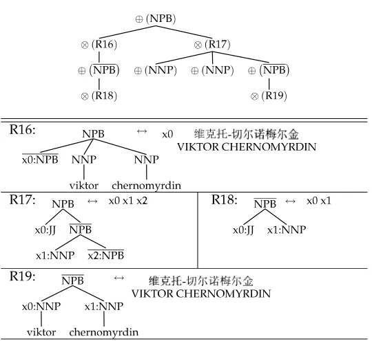
Condition 1: If we reach an additive e-forest node, for each of its children, which are multiplicative e-forest nodes, we go to condition 2 to recursively extract rules from it to obtain a set of multiplicative derivation-forest nodes, respectively. We form an additive derivation-forest node, and take these newly produced multiplicative derivation-forest nodes (by going to condition 2) as children. After this, we return the additivederivation-forest node.
[image:11.486.53.323.375.623.2]For instance, at node⊕1(NPB) in Figure 7, for each of its children, e-forest nodes⊗2(NPB) and⊗11(NPB), we go to condition 2 to extract rules on it, to form multiplicative derivation forest nodes,⊗(R16) and⊗(R17) in Figure 8.
r
Condition 2: If we reach a multiplicative e-forest node, we extract a set of rules rooted at it using the procedure in Galley et al. (2006); and for each rule, we form a multiplicative derivation-forest node, and go to condition 1 to form the additive derivation-forest nodes for the additive frontier e-forest nodes of the newly extracted rule, and then make these additive derivation-forest nodes the children of the multiplicative derivation-forest node. After this, we return a set of multiplicative derivation-forest nodes, each corresponding to one rule extracted from the multiplicative e-forest node we just reached.Figure 8
For example, at node⊗11(NPB) in Figure 7, we extract a rule from it and form derivation-forest node⊗(R17) in Figure 8. We then go to condition 1 to obtain, for each of the additive frontier e-forest nodes (in Figure 7) of this rule, a derivation-forest node, namely,⊕(NNP),⊕(NNP), and⊕(NPB) in Figure 8. We make these derivation-forest⊕-nodes the children of derivation-forest node⊗(R17).
This procedure transforms the packed e-forest in Figure 7 into a packed synchro-nous derivation in Figure 8. This algorithm is an extension of the extraction algorithm in Galley et al. (2006), in the sense that we have an extra condition (1) to relay rule extraction on additive e-forest nodes.
The forest-based rule extraction algorithm produces much larger grammars than the tree-based one, making it difficult to scale to very large training data. From a 50M-word Chinese-to-English parallel corpus, we can extract more than 300 million translation rules, while the tree-based rule extraction algorithm gives approximately 100 million. However, the restructured trees from the simple binarization methods are not guaranteed to give the best trees for syntax-based machine translation. What we desire is a binarization method that still produces single parse trees, but is able to mix left binarization and right binarization in the same tree. In the following, we use the EM algorithm to learn the desirable binarization on the forest of binarization alternatives proposed by the parallel binarization algorithm.
3.4 Learning How to Binarize Via the EM Algorithm
The basic idea of applying the EM algorithm to choose a re-structuring is as follows. We perform a set{β}of binarization operations on a parse treeτ. Each binarizationβis the sequence of binarizations on the necessary (i.e., factorizable) nodes inτin pre-order. Each binarization βresults in a restructured treeτβ. We extract rules from (τβ,f,a), generating a translation model consisting of parameters (i.e., rule probabilities)θ. Our aim is to first obtain the rule probabilities that are the maximum likelihood estimate of the training tuples, and then produce the Viterbi binarization tree for each training tuple.
The probability P(τβ,f,a) of a (τβ,f,a)-tuple is what the basic syntax-based trans-lation model is concerned with. It can be further computed by aggregating the rule probabilities P(r) in each derivationωin the set of all derivationsΩ(Galley et al. 2004). That is,
P(τβ,f,a)=
ω∈Ω
r∈ω
P(r) (1)
The rule probabilities are estimated by the inside–outside algorithm (Lari and Young 1990; Knight, Graehl, and May 2008), which needs to run on derivation forests. Our previous sections have already presented algorithms to transform a parse tree into a binarization forest, and then transform the (e-forest,f,a)-tuples into derivation forests (e.g., Figure 8), on which the inside–outside algorithm can then be applied.
of the node corresponding to the r. Each rule node (or multiplicative node) dom-inates several other additive children nodes, and we present the ith child node as
childi(r), among the total number ofnchildren. For example, in Figure 8, for the ruler
corresponding to the left child of the forest root (labeled asNPB),parent(r) isNPB, and
child1(NPB)=r. Based on these notations, we can compute the inside probabilityα(A) of an additive node labeled asAand the outside probabilityβ(B) of an additive forest node labeled asBas follows.
α(A)=
r∈{child(A)}
P(r)×
i=1...n
α(childi(r)) (2)
β(B)=
r:B∈{child(r)}
P(r)×β(parent(r))×
C∈{child(r)}−{B}
α(C) (3)
In the expectation step, the contribution of each occurrence of a rule in a derivation-forest to the total expected count of that rule is computed as
β(parent(r))×P(r)×
i=1...n
α(childi(r)) (4)
In the maximization step, we use the expected counts of rules, #r, to update the proba-bilities of the rules.
P(r)= #r
rule q:root(q)=root(r)#q
(5)
[image:13.486.114.429.157.219.2]Because it is well known that applying EM with tree fragments of different sizes causes overfitting (Johnson 1998a), and because it is also known that syntax MT models with larger composed rules in the mix significantly outperform rules that minimally explain the training data (minimal rules) in translation accuracy (Galley et al. 2006), we use minimal rules to construct the derivation forests from (e-binarization-forest,f,a )-tuples during running of the EM algorithm, but, after the EM re-structuring is finished, we build the final translation model using composed rules for MT evaluation.
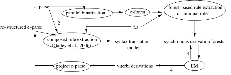
[image:13.486.54.448.510.638.2]Figure 9 is the actual pipeline that we use for EM binarization. We first generate a packed e-forest via parallel binarization. We then extract minimal translation rules from
Figure 9
the (e-forest,f,a)-tuples, producing synchronous derivation forests. We run the inside– outside algorithm on the derivation forests until convergence. We obtain the Viterbi derivations and project the English parses from the derivations. Finally, we extract composed rules using Galley et al. (2006)’s (e-tree,f,a)-based rule extraction algorithm.
When extracting composed rules from (e-parse, f, a)-tuples, we use an “ignoring-X -node” trick to the rule extraction method in Galley et al. (2006) to avoid breaking the local dependencies captured in complex rules. The trick is that new nodes introduced by binarization are not counted when computing the rule size limit unless they appear as the rule roots. The motivation is that newly introduced nodes break the local depen-dencies, deepening the parses. In Galley et al., a composed rule is extracted only if the number of internal nodes it contains does not exceed a limit, similar to the phrase length limit in phrase-based systems. This means that rules extracted from the restructured trees will be smaller than those from the unrestructured trees, if theXnodes are deleted from the rules. As shown in Galley et al., smaller rules lose context, and thus give lower translation accuracy. IgnoringXnodes when computing the rule sizes preserves the unrestructured rules in the resulting translation model and adds substructures as bonuses.
3.5 Experimental Results
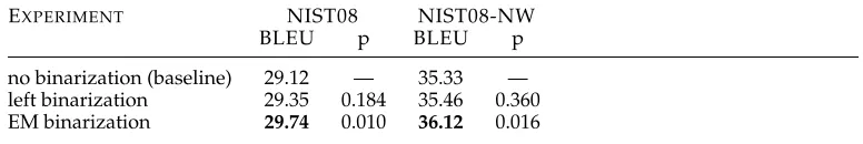
We carried out experiments to evaluate different tree binarization methods in terms of translation accuracy for Chinese-to-English translation. The baseline syntax MT sys-tem was trained on the original, non-restructured trees. We also built one MT syssys-tem by training on left-binarizations of training trees, and another by training on EM-binarizations of training trees.
Table 1 shows the results on end-to-end MT. The bootstrap p-values were computed for the pairwise BLEU comparison between the EM binarization and the baseline. The results show that tree binarization improves MT system accuracy, and that EM binariza-tion outperforms left binarizabinariza-tion. The results also show that the EM re-structuring sig-nificantly outperforms (p<0.05) the no re-structuring baseline on the NIST08 eval set.
[image:14.486.46.434.599.664.2]The MT improvement by tree re-structuring is also validated by our previous work (Wang, Knight, and Marcu 2007), in which we reported a 1 BLEU point gain from EM binarization under other training/testing conditions; other simple binarization methods were examined in that work as well, showing that simple binarizations also improve MT accuracy, and that EM binarization consistently outperforms the simple binarization methods.
Table 1
Translation accuracy versus binarization algorithms. In this and all other tables reporting BLEU performance, statistically significant improvements over the baseline are highlighted. p = the paired bootstrap p-value computed between each system and the baseline, showing the level at which the two systems are significantly different.
EXPERIMENT NIST08 NIST08-NW
BLEU pBLEU p
Table 2
# admissible nodes, # rules versus re-structuring methods.
RE-STRUCTURING METHOD # ADMISSIBLENODES(M) # RULES(M)
no binarization 13 76.0
left binarization 17.2 153.4
EM binarization 17.4 154.8
We think that these improvements are explained by the fact that tree re-structuring introduces more admissible trees nodes in the training trees and enables the forming of additional rules. As a result, re-structuring produces more rules. Table 2 shows the number of admissible nodes made available by each re-structuring method, as well as by the baseline. Table 2 also shows the sizes of the resulting grammars.
The EM binarization is able to introduce more admissible nodes because it mixes both left and right binarizations in the same tree. We computed the binarization biases learned by the EM algorithm for each nonterminal from the binarization forest of parallel head binarizations of the training trees (Table 3). Of course, the binarization bias chosen by left-/right-binarization methods would be 100% deterministic. One noticeable message from Table 3 is that most of the categories are actually biased toward left-binarization. The reason might be that the head sub-constituents of most English categories tend to be on the left.
[image:15.486.55.436.508.665.2]Johnson (1998b) argues that the more nodes there are in a treebank, the stronger the independence assumptions implicit in the PCFG model are, and the less accurate the estimated PCFG will usually be—more nodes break more local dependencies. Our experiments, on the other hand, show MT accuracy improvement by introducing more admissible nodes. This initial contradiction actually makes sense. The key is that we use composed rules to build our final MT system and that we introduce the “ignoring-X -node” trick to preserve the local dependencies. More nodes in training trees weaken the accuracy of a translation model of minimal rules, but boost the accuracy of a translation model of composed rules.
Table 3
Binarization bias learned by the EM re-structuring method on the model 4 word alignments.
nonterminal left-binarization (%) right-binarization (%)
NP 98 2
NPB 1 99
VP 95 5
PP 86 14
ADJP 67 33
ADVP 76 24
S 94 6
S-C 17 83
SBAR 93 7
QP 89 11
WHNP 98 2
SINV 94 6
4. Re-Labeling Trees for Training
The syntax translation model explains (e-parse, f, a)-tuples by a series of applications of translation rules. At each derivation step, which rule to apply next depends only on the nonterminal label of the frontier node being expanded. In the Penn Treebank annotation, the nonterminal labels are too coarse to encode enough context information to accurately predict the next translation rule to apply. As a result, using the Penn Treebank annotation can license ill-formed subtrees (Figure 10). This subtree contains an error that induces a VP as an SG-C when the head of the VP is the finite verb dis-cussed.The translation error leads to the ungrammatical “... confirmed discussed ...”. This translation error occurs due to the fact that there is no distinction between finite VPs and non-finite VPs in Penn Treebank annotation. Monolingual parsing suffers similarly, but to a lesser degree.
Re-structuring of training trees enables the reuse of sub-constituent structures, but further introduces new nonterminals and actually reduces the context for rules, thus making this “coarse nonterminal” problem more severe. In Figure 11, R23 may be extracted from a construct like S(S CC S) via tree binarization, and R24 may be extracted from a construct like S(NP NP-C VP) via tree binarization. Composing R23 and R24 forms the structure in Figure 11(b), which, however, is ill-formed. This wrong structure in Figure 11(b) yields ungrammatical translations like he likes reading she does not like reading. Tree binarization enables the reuse of substructures, but causes over-generation of trees at the same time.
We solve the coarse-nonterminal problem by refining/re-labeling the training tree labels. Re-labeling is done by enriching the nonterminal label of each tree node based on its context information.
[image:16.486.48.394.446.625.2]Re-labeling has already been used in monolingual parsing research to improve parsing accuracy of PCFGs. We are interested in two types of re-labeling methods: Linguistically motivated re-labeling (Klein and Manning 2003; Johnson 1998b) enriches the labels of parser training trees using parent labels, head word tag labels, and/or sibling labels. Automatic category splitting (Petrov et al. 2006) refines a nonterminal
Figure 10
Figure 11
Tree binarization over-generalizes the parse tree. Translation rules R23 and R24 are acquired from binarized training trees, aiming for reuse of substructures. Composing R23 and R24, however, results in an ill-formed tree. The new nonterminal S introduced in tree binarization needs to be refined into different sub-categories to prevent R23 and R24 from being composed. Automatic category splitting can be employed for refining the S.
by classifying the nonterminal into a fine-grained sub-category, and this sub-classing is learned via the EM algorithm. Category splitting is realized by several splitting-and-merging cycles. In each cycle, the nonterminals in the PCFG rules are split by splitting each nonterminal into two. The EM algorithm is employed to estimate the split PCFG on the Penn Treebank training trees. After that, 50% of the new nonterminals are merged based on some loss function, to avoid overfitting.
4.1 Linguistic Re-labeling
In the linguistically motivated approach, we employ the following set of rules to re-label tree nodes. In our MT training data:
r
SPLIT-VP: annotates each VP nodes with its head tag, and then merges allfinite VP forms to a single VPF.
r
SPLIT-IN: annotates each IN node with the combination of IN and its parent node label. IN is frequently overloaded in the Penn Treebank. For instance, its parent can be PP or SBAR.These two operations re-label the tree in Figure 12(a1) to Figure 12(b1). Example rules extracted from these two trees are shown in Figure 12(a2) and Figure 12(b2), respectively. We apply this re-labeling on the MT training tree nodes, and then acquire rules from these re-labeled trees. We chose to split only these two categories because our syntax MT system tends to frequently make parse errors in these two categories, and because, as shown by Klein and Manning (2003), further refining the VP and IN categories is very effective in improving monolingual parsing accuracy.
This type of re-labeling fixes the parse error in Figure 10. SPLIT-VP transforms the R18 root to VPF, and the R17 frontier node to VP.VBN. Thus R17 and R18 can never be composed, preventing the wrong tree being formed by the translation model.
4.2 Statistical Re-labeling
Figure 12
their parser to directly produce category-split parse trees for the MT training data, we separate the parsing step and the re-labeling step. The re-labeling method is as follows.
1. Run a parser to produce the MT training trees.
2. Binarize the MT training trees via the EM binarization algorithm. 3. Learn ann-way split PCFG from the binarized trees via the algorithm
described in Petrov et al. (2006).
4. Produce the Viterbi split annotations on the binarized training trees with the learned category-split PCFG.
As we mentioned earlier, tree binarization sometimes makes the decoder over-generalize the trees in the MT outputs, but we still binarize the training trees before performing category splitting, for two reasons. The first reason is that the improve-ment on MT accuracy we achieved by tree re-structuring indicates that the benefit we obtained from structure reuse triumphs the problem of tree over-generalization. The second is that carrying out category splitting on unbinarized training trees blows upthe grammar—splitting a CFG rule of rank 10 results in 211 split rules. This re-labeling procedure tries to achieve further improvement by trying to fix the tree over-generalization problem of re-structuring while preserving the gain we have already obtained from tree re-structuring.
Figure 12(c1) shows a category-split tree, and Figure 12(c2) shows the minimal xRs rules extracted from the split tree. In Figure 12(c2), the two VPs (VP-0 and VP-2) now belong to two different categories and cannot be used in the same context.
In this re-labeling procedure, we separate the re-labeling step from the parsing step, rather than using a parser like the one in Petrov et al. (2006) to directly produce category-split parse trees on the English corpus. We think that we benefit from this separation in the following ways: First, this gives us the freedom to choose the parser to produce the initial trees. Second, this enables us to train the re-labeler on the domains where the MT system is trained, instead of on the Penn Treebank. Third, this enables us to choose our own tree binarization methods.
[image:19.486.53.438.587.663.2]Tree re-labeling fragments the translation rules. Each refined rule now fits in fewer contexts than its corresponding coarse rule. Re-labeling, however, does not explode the grammar size, nor does re-labeling deteriorate the reuse of substructures. This is because the re-labeling (whether linguistic or automatic) results in very consistent annotations. Table 4 shows the sizes of the translation grammars from different re-labelings of the training trees, as well as that from the unrelabeled ones.
Table 4
Grammar size vs. re-labeling methods. Re-labeling does not explode the grammar size.
RE-LABELING METHOD #RULES(M) NONTERMINAL SET SIZE
No re-labeling 154.80 144
Linguistically motivated re-labeling 154.97 210
4-way splitting (90% merging) 158.89 178
8-way splitting (90% merging) 160.62 195
It would be very interesting to perform automatic category splitting with synchro-nous translation rules and run the EM algorithm on the synchrosynchro-nous derivation forests. Synchronous category splitting is computationally much more expensive, so we do not study it here.
4.3 Experimental Results
[image:20.486.52.433.582.664.2]We ran end-to-end MT experiments by re-labeling the MT training trees. Our two base-line systems were a syntax MT system with neither re-structuring nor re-labeling, and a syntax MT system with re-structuring but no re-labeling. The linguistically motivated re-labeling method was applied directly on the original (unrestructured) training trees, so that it could be compared to the first baseline. The automatic category splitting re-labeling method was applied to binarized trees so as to avoid the explosion of the split grammar, so it is compared to the second baseline. The experiment results are shown in Table 5.
Both labeling methods helpMT accuracy. Putting both structuring and re-labeling together results in 0.93 BLEU points improvement on NIST08 set, and 1 BLEU point improvement on the newswire subset. All p-values are computed between the re-labeling systems and Baseline1. The improvement made by the linguistically moti-vated re-labeling method is significant at the 0.05 level. Because the automatic category splitting is carried out on the top of EM re-structuring and because, as we have already shown, EM structuring significantly improves Baseline1, putting them together re-sults in better translations with more confidence.
If we compare these results to those in Table 1, we notice that re-structuring tends to helpMT accuracy more than re-labeling. We mentioned earlier that re-structuring overgeneralizes structures, but enables reuse of substructures. Results in Table 5 and Table 1 show substructure reuse mitigates structure over-generalization in our tree re-structuring method.
5. Re-aligning (Tree, String) Pairs for Training
So far, we have improved the English structures in our parsed, aligned training corpus. We now turn to improving the word alignments.
Some MT systems use the same model for alignment and translation—examples include Brown et al. (1993), Wu (1997), Alshawi, Bangalore, and Douglas (1998), Yamada and Knight (2001, 2002), and Cohn and Blunsom (2009). Other systems use Brown et al. for alignment, then collect counts for a completely different model, such as Och and Ney
Table 5
Impact of re-labeling methods on MT accuracy as measured by BLEU. Four-way splitting was carried out on EM-binarized trees; thus, it already benefits from tree re-structuring. All p-values are computed against Baseline1.
EXPERIMENT NIST08 NIST08-NW
BLEU pBLEU p
Baseline1 (no re-structuring and no re-labeling) 29.12 — 35.33 — Linguistically motivated re-labeling 29.57 0.029 35.85 0.050
(2004) or Chiang (2007). Our basic syntax-based system falls into this second category, as we learn our syntactic translation model from a corpus aligned with word-based techniques. We would like to inject more syntactic reasoning into the alignment process. We start by contrasting two generative translation models.
5.1 The Traditional IBM Alignment Model
IBM Model 4 (Brown et al. 1993) learns a set of four probability tables to compute P(f|e) given a foreign sentence f and its target translation e via the following (simplified) generative story:
1. A fertilityyfor each wordeiineis chosen with probability Pfert(y|ei).
2. A null word is inserted next to each fertility-expanded word with probability Pnull.
3. Each tokeneiin the fertility-expanded word and null string is translated
into some foreign wordfiinf with probability Ptrans(fi|ei).
4. The position of each foreign wordfithat was translated fromeiis changed
by∆(which may be positive, negative, or zero) with probability
Pdistortion(∆|A(ei),B(fi)), whereAandBare functions over the source and target vocabularies, respectively.
Brown et al. (1993) describe an EM algorithm for estimating values for the four tables in the generative story. With those values in hand, we can calculate the highest-probability (Viterbi) alignment for any given string pair.
Two scale problems arise in this algorithm. The first is the time complexity of enu-merating alignments for fractional count collection. This is solved by considering only a subset of alignments, and by bootstrapping the Ptranstable with a simpler model that
admits fast count collection via dynamic programming, such as IBM Model 1 (Brown et al. 1993) or Aachen HMM (Vogel, Ney, and Tillmann 1996). The second problem is one of space. In theory, the initial Ptrans table contains a cell for every English word
paired with every Chinese word—this would be infeasible. Fortunately, in practice, the table can be initialized with only those word pairs observed co-occurring in the parallel training text.
5.2 A Syntax Re-alignment Model
Our syntax translation model learns a single probability table to compute P(etree,f) given a foreign sentence f and a parsed target translationetree. In the following gen-erative story we assume a starting variable with syntactic typev.
1. Choose a rulerto replacev, with probability Prule(r|v).
2. For each variable with syntactic typeviin the partially completed (tree,
string) pair, continue to choose rulesriwith probability Prule(ri|vi) to
replace these variables until there are no variables remaining.
with that (tree, string) pair yields the minimal rules of Figure 2. A different alignment yields different rules. Figure 13 shows two other alignments and their corresponding minimal rules. As noted before, a set of minimal rules in proper sequence forms a derivation tree of rules that explains the (tree, string) pair. Because rules explain variable-size fragments (e.g., R35 vs. R6), the possible derivation trees of rules that explain a sentence pair have varying sizes. The smallest such derivation tree has a single large rule (which does not appear in Figure 13). When our model chooses a particular derivation tree of minimal rules to explain a given (tree, string) pair it implicitly chooses the alignment that produced these rules as well.3Our model can choose a derivation by using any of the rules in Figures 13 and 2. We would prefer it select the derivation that yields the good alignment in Figure 1.
We can also develop an EM learning approach for this model. As in the IBM approach, we have both time and space issues. Time complexity, as we will see sub-sequently, is O(mn3), where mis the number of nodes in the English training tree and
n is the length of the corresponding Chinese string. Space is more of a problem. We would like to initialize EM with all the rules that might conceivably be used to explain the training data. However, this set is too large to practically enumerate.
To reduce the model space we first create a bootstrap alignment using a simpler word-based model. Then we acquire a set of minimal translation rules from the (tree, string, alignment) triples. Armed with these rules, we can discard the word-based alignments andre-alignwith the syntax translation model.
We summarize the approach described in this section as:
1. Obtain bootstrapalignments for a training corpus using word-based alignment.
2. Extract minimal rules from the corpus and alignments using GHKM, noting the partial alignment that is used to extract each rule.
3. Construct derivation forests for each (tree, string) pair, ignoring the alignments, and run EM to obtain Viterbi derivation trees, then use the annotated partial alignments to obtain Viterbi alignments.
4. Use the new alignments to re-train the full MT system, this time collecting composed rules as well as minimal rules.
5.3 EM Training for the Syntax Translation Model
Consider the example of Figure 13 again. The top alignment was the bootstrap align-ment, and thus prior to any experiment we obtained the corresponding indicated minimal rule set and derivation. This derivation is reasonable but there are some poorly motivated rules, from a linguistic standpoint. The Chinese wordÜÜÜ roughly means
the two shoresin this context, but the rule R35 learned from the alignment incorrectly includes between. However, other sentences in the training corpus have the correct
Figure 13
The minimal rules extracted from two different alignments of the sentence in Figure 1.
alignment, which yields rules in Figure 2, such as R8. Figure 2 also contains rules R4 and R6, learned from yet other sentences in the training corpus, which handle theóóó... ¥
¥¥structure (which roughly translates toin between), thus allowing a derivation which
contains the minimal rule set of Figure 2 and implies the alignment in Figure 1.
rules for the same situation over several sentences, if possible. R35 is a possible rule in 46 of the 329,031 sentence pairs in the training corpus, and R8 is a possible rule in 100 sentence pairs. Well-formed rules are more usable than ill-formed rules and the partial alignments behind these rules, generally also well-formed, become favored as well. The toprow of Figure 14 contains an example of an alignment learned by the bootstrapalignment model that includes an incorrect link. Rule R25, which is extracted from this alignment, is a poor rule. A set of commonly seen rules learned from other training sentences provide a more likely explanation of the data, and the consequent alignment omits the spurious link.
Figure 14
Table 6
Translation performance, grammar size versus the re-alignment algorithm proposed in Section 5.2, and re-alignment as modified in Section 5.4.
EXPERIMENT NIST08 NIST08-NW #RULES(M)
BLEU pBLEU p
no re-alignment (baseline) 29.12 — 35.33 — 76.0
EM re-alignment 29.18 0.411 35.52 0.296 75.1
EM re-alignment with size prior 29.37 0.165 35.96 0.050 110.4
Now we need an EM algorithm for learning the parameters of the rule set that
maximize
corpusP(tree,string). Knight, Graehl, and May (2008) present a generic such algo-rithm for tree-to-string transducers that runs in O(mn3) time, as mentioned earlier. The algorithm consists of two components: DERIV, which is a procedure for constructing a packed forest of derivation trees of rules that explain a (tree, string) bitext corpus given that corpus and a rule set, and TRAIN, which is an iterative parameter-setting procedure.
We initially attempted to use the top-down DERIValgorithm of Knight, Graehl, and May (2008), but as the constraints of the derivation forests are largely lexical, too much time was spent on exploring dead-ends. Instead we build derivation forests using the following sequence of operations:
1. Binarize rules using the synchronous binarization algorithm for tree-to-string transducers described in Zhang et al. (2006).
2. Construct a parse chart with a CKY parser simultaneously constrained on the foreign string and English tree, similar to the bilingual parsing of Wu (1997).4
3. Recover all reachable edges by traversing the chart, starting from the topmost entry.
Because the chart is constructed bottom-up, leaf lexical constraints are encountered immediately, resulting in a narrower search space and faster running time than the top-down DERIV algorithm for this application. The Viterbi derivation tree tells us which English words produce which Chinese words, so we can extract a word-to-word alignment from it.
Although in principle the re-alignment model and translation model learn parame-ter weights over the same rule space, in practice we limit the rules used for re-alignment to the set of minimal rules.
5.4 Adding a Rule Size Prior
An initial re-alignment experiment shows a small rise in BLEU scores from the baseline (Table 6), but closer inspection of the rules favored by EM implies we can do even better.
EM has a tendency to favor a few large rules over many small rules, even when the small rules are more useful. Referring to the rules in Figures 2 and 13, note that possible derivations for (taiwan’s,ÑÑÑlll)
5are R33, R2–R3, and R38–R40. Clearly the third deriva-tion is not desirable, and we do not discuss it further. Between the first two derivaderiva-tions, R2–R3 is preferred over R33, as the conditioning for possessive insertion is not related to the specific Chinese word being inserted. Of the 1,902 sentences in the training corpus where this pair is seen, the bootstrap alignments yield the R33 derivation 1,649 times and the R2–R3 derivation 0 times. Re-alignment does not change the result much; the new alignments yield the R33 derivation 1,613 times and again never choose R2–R3. The rules in the second derivation themselves are not rarely seen—R2 is in 13,311 forests
otherthan those where R33 is seen, and R3 is in 2,500 additional forests. EM gives R2 a probability ofe−7.72—better than 98.7% of rules, and R3 a probability ofe−2.96. But R33 receives a probability ofe−6.32and is preferred over the R2–R3 derivation, which has a combined probability ofe−10.68.
The preference for shorter derivations containing large rules over longer derivations containing small rules is due to a general tendency for EM to prefer derivations with few atoms. Marcu and Wong (2002) note this preference but consider the phenomenon a feature, rather than a bug. Zollmann and Sima’an (2005) combat the overfitting aspect for parsing by using a held-out corpus and a straight maximum likelihood estimate, rather than EM. DeNero, Bouchard-C ˆot´e, and Klein (2008) encourage small rules with a modeling approach; they put a Dirichlet process prior of rule size over their model and learn the parameters of the geometric distribution of that prior with Gibbs sampling. We use a simpler modeling approach to accomplish the same goals as DeNero, Bouchard-C ˆot´e, and Klein which, although less elegant, is more scalable and does not require a separate Bayesian inference procedure.
As the probability of a derivation is determined by the product of its atom probabil-ities, longer derivations with more probabilities to multiply have an inherent disadvan-tage against shorter derivations, all else being equal. EM is an iterative procedure and thus such a bias can lead the procedure to converge with artificially raised probabilities for short derivations and the large rules that constitute them. The relatively rare ap-plicability of large rules (and thus lower observed partial counts) does not overcome the inherent advantage of large coverage. To combat this, we introduce size terms into our generative story, ensuring that all competing derivations for the same sentence contain the same number of atoms:
1. Choose a rule sizeswith costcsize(s)s−1.
2. Choose a ruler(of sizes) to replace the start symbol with probability Prule(r|s,v).
3. For each variable in the partially completed (tree, string) pair, continue to choose sizes followed by rules, recursively to replace these variables until there are no variables remaining.
This generative story changes the derivation comparison from R33 vs. R2–R3 to S2– R33 vs. R2–R3, where S2 is the atom that represents the choice of size 2 (the size of a rule
in this context is the number of non-leaf and non-root nodes in its tree fragment). Note that the variable number of inclusions implied by the exponent in the generative story above ensures that all derivations have the same size. For example, a derivation with one size-3 rule, a derivation with one size-2 and one size-1 rule, and a derivation with three size-1 rules would each have three atoms. With this revised model that allows for fair comparison of derivations, the R2–R3 derivation is chosen 1,636 times, and S2–R33 is not chosen. R33 does, however, appear in the translation model, as the expanded rule extraction described in Section 1 creates R33 by joining R2 and R3.
The probability of size atoms, like that of rule atoms, is decided by EM. The revised generative story tends to encourage smaller sizes by virtue of the exponent. This does not, however, simply ensure the largest number of rules per derivation is used in all cases. Ill-fitting and poorly motivated rules such as R42, R43, and R44 in Figure 13 are not preferred over R8, even though they are smaller. However, R6 and R8 are preferred over R35, as the former are useful rules. Although the modified model does not sum to 1, it can nevertheless lead to an improvement in BLEU score.
5.5 Experimental Results
The end-to-end MT experiment used as baseline and described in Sections 3.5 and 4.3 was trained on IBM Model 4 word alignments, obtained by running GIZA, as described in Section 2. We compared this baseline to an MT system that used alignments obtained by re-aligning the GIZA alignments using the method of Section 5.2 with the 36 million word subset of the training corpus used for re-alignment learning. We next compared the baseline to an MT system that used re-alignments obtained by also incorporating the size prior described in Section 5.4. As can be seen by the results in Table 6, the size prior method is needed to obtain reasonable improvement in BLEU. These results are consistent with those reported in May and Knight (2007), where gains in Chinese and Arabic MT systems were observed, though over a weaker baseline and with less training data than is used in this work.
6. Combining Techniques
We have thus far seen gains in BLEU score by independent improvements in training data tree structure, syntax labeling, and alignment. This naturally raises the question of whether the techniques can be combined, that is, if improvement in one aspect of training data aids in improvement of another. As reported in Section 4.3 and Table 5, we were able to improve re-labeling efforts and take advantage of the split-and-merge technique of Petrov et al. (2006) by first re-structuring via the method described in Sec-tion 3.4. It is unlikely that such re-structuring or re-labeling would aid in a subsequent re-alignment procedure like that of Section 5.2, for re-structuring changes trees based on a given alignment, and re-alignment can only change links when multiple instances of a (subtree, substring) tuple are found in the data with different partial alignments. Re-structuring beforehand changes the trees over different alignments differently. It is unlikely that many (subtree, substring) tuples with more than one partial alignment would remain after a re-structuring.
Table 7
Summary of experiments in this article, including a combined experiment with re-alignment, re-structuring, and re-labeling.
EXPERIMENT NIST08 NIST08-NW #RULES(M)
BLEU pBLEU p
Baseline (no binarization, no re-labeling, 29.12 — 35.33 — 76.0 Model 4 alignments)
left binarization 29.35 0.184 35.46 0.360 153.4
EM binarization 29.74 0.010 36.12 0.016 154.8
Linguistic re-labeling 29.57 0.029 35.85 0.050 154.97 EM binarization + EM re-labeling 30.05 0.001 36.42 0.003 158.89
(4-way splitting w/ 90% merging)
EM re-alignment 29.18 0.411 35.52 0.296 75.1
Size prior EM re-alignment 29.37 0.165 35.96 0.050 110.4
Size prior EM re-alignment + 30.6 0.001 36.73 0.002 222.0 EM binarization + EM re-labeling
Better re-structuring should in turn lead to better re-labeling, and this should increase the performance of the overall MT pipeline.
To test this hypothesis we pprocessed alignments using the modified re-alignment procedure described in Section 5.4. We next used those re-alignments to obtain new binarizations of trees following the EM binarization method described in Sec-tion 3.4. Finally, re-labeling was done on these binarized trees using 4-way splitting with 90% merging, as described in Section 4. The final trees, along with the alignments used to get these trees and of course the parallel Chinese sentences, were then used as the training data of our MT pipeline. The results of this combined experiment are shown in Table 7 along with the other experiments from this article, for ease of comparison. As can be seen from this table, the progressive improvement of training data leads to an overall improvement in MT system performance. As noted previously, there tends to be a correspondence between the number of unique rules extracted and MT performance. The final combined experiment has the greatest number of unique rules. The improvements made to syntax and alignment described in this article unify these two independently determined annotations over the bitext, and this thus leads to more admissible nodes and a greater ability to extract rules. Such a unification can lead to over-generalization, as rules lacking sufficient context may be extracted and used to the system’s detriment. This is why a re-labeling technique is also needed, to ensure that sufficient rule specificity is maintained.
7. Conclusion
the training data used in the original MT task and are thus applicable to a string-to-tree MT system for any language pair.
Acknowledgments
Some of the results in this article appear in Wang, Knight, and Marcu (2007) and May and Knight (2007). The linguistically motivated re-labeling method is due to Steve DeNeefe, Kevin Knight, and David Chiang. The authors also wish to thank Slav Petrov for his helpwith the Berkeley parser, and the anonymous reviewers for their helpful comments. This research was supported under DARPA Contract No. HR0011-06-C-0022, BBN subcontract 9500008412.
References
Alshawi, Hiyan, Srinivas Bangalore, and Shona Douglas. 1998. Automatic acquisition of hierarchical transduction models for machine translation. In
Proceedings of the 36th Annual Meeting of the Association for Computational Linguistics (ACL) and 17th International Conference on Computational Linguistics (COLING) 1998, pages 41–47, Montr´eal.
Brown, Peter F., Stephen A. Della Pietra, Vincent J. Della Pietra, and Robert L. Mercer. 1993. The mathematics of statistical machine translation: Parameter estimation.Computational Linguistics, 19(2):263–312.
Charniak, Eugene. 2000. A maximum-entropy-inspired parser. InProceedings of the 1st North American Chapter of the Association for Computational Linguistics Conference (NAACL), pages 132–139, Seattle, WA.
Chiang, David. 2007. Hierarchical phrase-based translation.Computational Linguistics, 33(2):201–228.
Cohn, Trevor and Phil Blunsom. 2009. A Bayesian model of syntax-directed tree to string grammar induction. In
Proceedings of the 2009 Conference on Empirical Methods in Natural Language Processing, pages 352–361, Singapore. Collins, Michael. 1997. Three generative,
lexicalized models for statistical parsing. InProceedings of the 35th Annual Meeting of the Association for Computational Linguistics (ACL), pages 16–23, Madrid.
Dempster, Arthur P., Nan M. Laird, and Donald B. Rubin. 1977. Maximum likelihood from incomplete data via the EM algorithm.Journal of the Royal Statistical Society, 39(1):1–38.
DeNeefe, Steve, Kevin Knight, Wei Wang, and Daniel Marcu. 2007. What can syntax-based MT learn from phrase-based MT? InProceedings of EMNLP–CoNLL-2007, pages 755–763, Prague.
DeNero, John, Alexandre Bouchard-C ˆot´e, and Dan Klein. 2008. Sampling alignment structure under a Bayesian translation model. InProceedings of the 2008 Conference on Empirical Methods in Natural Language Processing (EMNLP), pages 314–323, Honolulu, HI.
Gale, William A. and Geoffrey Sampson. 1996. Good-Turing frequency estimation without tears.Journal of Quantitative Linguistics, 2(3):217–237.
Galley, Michel, Jonathan Graehl, Kevin Knight, Daniel Marcu, Steve DeNeefe, Wei Wang, and Ignacio Thayer. 2006. Scalable inference and training of context-rich syntactic translation models. InProceedings of the 21st International Conference on Computational Linguistics (COLING) and 44th Annual Meeting of the Association for Computational Linguistics (ACL), pages 961–968, Sydney.
Galley, Michel, Mark Hopkins, Kevin Knight, and Daniel Marcu. 2004. What’s in a translation rule? InProceedings of the Human Language Technology Conference and the North American Association for
Computational Linguistics (HLT-NAACL), pages 273–280, Boston, MA.
Good, Irving J. 1953. The population frequencies of species and the estimation of population parameters.Biometrika, 40(3):237–264.
Goodman, Joshua. 1999. Semiring parsing.
Computational Linguistics, 25(4):573–605. Huang, Bryant and Kevin Knight. 2006.
Relabeling syntax trees to improve syntax-based machine translation accuracy. InProceedings of the main conference on Human Language Technology Conference of the North American Chapter of the Association of Computational Linguistics (NAACL-HLT), pages 240–247, New York, NY.
Johnson, Mark. 1998a. The DOP estimation method is biased and inconsistent.
Computational Linguistics, 28(1):71–76. Johnson, Mark. 1998b. PCFG models of
linguistic tree representations.
Computational Linguistics, 24(4):613–632. Klein, Dan and Chris Manning. 2003.