Applications of Lexicographic Semirings to Problems in Speech and Language Processing

Problems in Speech and Language Processing

Richard Sproat

Mahsa Yarmohammadi

Izhak Shafran

Oregon Health & Science University

Brian Roark

This article explores lexicographic semirings and their application to problems in speech and language processing. Specifically, we present two instantiations of binary lexicographic semirings, one involving a pair of tropical weights, and the other a tropical weight paired with a novel string semiring we term the categorial semiring. The first of these is used to yield an exact encoding of backoff models with epsilon transitions. Thislexicographic language model semiringallows for off-line optimization of exact models represented as large weighted finite-state transducers in contrast to implicit (on-line) failure transition representations. We present empirical results demonstrating that, even in simple intersection scenarios amenable to the use of failure transitions, the use of the more powerful lexicographic semiring is competitive in terms of time of intersection. The second of these lexicographic semirings is applied to the problem of extracting, from a lattice of word sequences tagged for part of speech, only the single best-scoring part of speech tagging for each word sequence. We do this by incorporating the tags as a categorial weight in the second component of ahTropical, Categorialilexicographic semiring, determinizing the resulting word lattice acceptor in that semiring, and then mapping the tags back as output labels of the word lattice transducer. We compare our approach to a competing method due to Povey et al. (2012).

1. Introduction

Applications of finite-state methods to problems in speech and language processing have grown significantly over the last decade and a half. From their beginnings in the

∗Google Inc., 76 Ninth Ave, 4th Floor, New York, NY 10011, USA. E-mail:{rws,roark}@google.com. ∗∗Center for Spoken Language Understanding, Oregon Health & Science University, 3181 SW Sam Jackson

Park Rd, GH40, Portland, OR 97239-3098, USA. E-mails:{mahsa.yarmohamadi,zakshafran}@gmail.com.

Submission received: 1 March 2013; revised version received: 5 November 2013; accepted for publication: 23 December 2013.

1950s and 1960s to implement small hand-built grammars (e.g., Joshi and Hopely 1996) through their applications in computational morphology in the 1980s (Koskenniemi 1983), finite-state models are now routinely applied in areas ranging from parsing (Abney 1996), to machine translation (Bangalore and Riccardi 2001; de Gispert et al. 2010), text normalization (Sproat 1996), and various areas of speech recognition includ-ing pronunciation modelinclud-ing and language modelinclud-ing (Mohri, Pereira, and Riley 2002).

The development of weighted finite state approaches (Mohri, Pereira, and Riley 2002; Mohri 2009) has made it possible to implement models that can rank alternative analyses. A number of weight classes—semirings—can be defined (Kuich and Salomaa 1986; Golan 1999), though for all practical purposes nearly all actual applications use the tropical semiring, whose most obvious instantiation is as a way to combinenegative log probabilitiesof words in a hypothesis in speech recognition systems. With few exceptions (e.g., Eisner 2001), there has been relatively little work on exploring applications of different semirings, in particularstructured semiringsconsisting of tuples of weights.

In this article we explore the use of what we termlexicographic semirings, which are tuples of weights where the comparison between a pair of tuples starts by comparing the first element of the tuple, then the second, and so forth until unequal values are found—just as lexicographic order is determined between words. We investigate two such lexicographic semirings, one based on pairs of tropical weights, and the other that uses a tropical weight paired with a novel string weight that we call thecategorial semiring. The latter is based loosely on the operations of categorial grammar.

We use the first semiring to provide an exact encoding of language models as weighted finite-state transducers using epsilon arcs in place of failure arcs. The sec-ond we apply to the problem of selecting only the single-best tagging for each word sequence in a tagged lattice. In each case we formally justify the application and demon-strate the correctness and efficiency on real domains.

1.1 Definitions

Adopting the notations often used in the speech and language literature (Mohri 2009), a semiring is a 4-tuple (K,⊕,⊗, ¯0, ¯1) with a nonempty set K on which two binary operations are defined, namely, the semiring plus⊕and semiring times⊗, such that:

1. (K,⊕) is a commutative monoid with identity ¯0;

2. (K,⊗) is a monoid with identity ¯1;

3. ⊗distributes over⊕; and

4. ¯0⊗k=k⊗¯0= ¯0 ∀k∈K.

Typically, ¯16= ¯0 is assumed, to avoid trivial semirings. Thetropical semiringis an example of a well-known semiring and is defined as (< ∪ {∞},min,+,∞, 0).

A weighted finite-state automaton or transducer isdeterministicorsubsequential if no two transitions leaving the same state have the same input label. Ageneric deter-minization algorithmcan transform a weighted finite-state acceptor or transducer into its deterministic form if such a form exists. For details on the algorithm and conditions for determinization, see Section 6.2 in Mohri (2009). The condition most relevant for our purpose is that the algorithm works with anyweakly divisiblesemiring. Briefly, a semiring (K,⊕,⊗, ¯0, ¯1) is said to bedivisibleif all non-¯0 elements admit an inverse, that is, (K−¯0) is a group. A semiring isweakly divisible if for anyx and y in Ksuch that x⊕y6=¯0 there exists at least onezsuch that (x⊕y)⊗z=x. The⊗iscancellativeifzis unique and can be written asz=(x⊕y)−1_{x. The non-unique case is not relevant here.}

1.2 Lexicographic Semirings

The notion ofweightcan be extended to complex tuples of weights, and semirings over those tuples. Of interest to us here is a tuple-based semiring, thelexicographic semiring.

A hW1,W2. . .Wni-lexicographic weight is a tuple of weights where each of the

weight classes W1,W2. . .Wn, must observe the path property (Mohri 2002). The path

property of a semiringKis defined in terms of thenatural orderonKsuch that:a<_Kbiff a⊕b=a. The tropical semiring mentioned above is a common example of a semiring that observes the path property, since

w1⊕w2 =min{w1,w2}

and therefore ifw1<Kw2, thenw1⊕w2=w1, and vice versa.

A particular instance of a lexicographic semiring, one that we will be making use of in this article, involves a pair of tropical weights, which we will notate thehT,Ti -lexicographic semiring. For this semiring the operations⊕and⊗are defined as follows (Golan 1999, pages 223–224):

hw1,w2i ⊕ hw3,w4i=

hw1,w2i ifw1 <w3or (w1 =w3&w2 <w4) hw3,w4i otherwise

hw1,w2i ⊗ hw3,w4i=hw1+w3,w2+w4i (1)

The termlexicographicis an apt term for this semiring because the comparison for⊕

is like the lexicographic comparison of strings, comparing the first elements, then the second, and so forth. Lexicographic semirings can be defined with other underlying semirings or tuple lengths.

1.3 An Example Application of Lexicographic Semiring: Implementing Ranking in Optimality Theory

As an example of a lexicographic semiring that has a tuple length (usually) greater than 2, consider one way in which one might implement constraint ranking in Optimality Theory.

Consider the following recent example from http://en.wikipedia.org/wiki/ Optimality_theory#Example: It accounts for the form of the regular noun plural suffix in English, which is voiceless /s/ after a voiceless stop (cats), /@z/ after a sibilant (dishes), and /z/ otherwise. Quoting directly from the Wikipedia example, the following constraints in the order given account for the phenomena:

1. *SS- Sibilant-Sibilant clusters are ungrammatical: one violation for every pair of adjacent sibilants in the output.

2. Agree(Voi)- Agree in specification of [voi]: one violation for every pair of adjacent obstruents in the output which disagree in voicing.

3. Max- Maximize all input segments in the output: one violation for each segment in the input that does not appear in the output. (This constraint prevents deletion.)

4. Dep- Output segments are dependent on having an input correspondent: one violation for each segment in the output that does not appear in the input. (This constraint prevents insertion.)

5. Ident(Voi)- Maintain the identity of the [voi] specification: one violation for each segment that differs in voicing between the input and output.

Consider the example ofdishes. From a presumed underlying form ofdish+z, GEN

generates a range of possible forms, including those in the lefthand column in the following table:

dish+z *SS Agree Max Dep Ident

Rdishiz *

dishis * *!

dishz *! *

dish *!

dishs *! *

Asterisks indicate violations, and exclamation marks indicate the critical violation that rules out the particular form. Bothdishsanddishzhave violations of*SS, and because none of the other forms violate*SS, and*SSis highest ranked, those two violations are critical. Concomitantly, any other violations (e.g.,dishsviolation ofIdent) are irrelevant for determining the fate of those forms. Moving down the constraint hierarchy, dish violates Max, because the suffix does not appear in this form; again this violation is critical, because the remaining two forms do not violate the constraint. Bothdishisand anddishizviolateDepbecause there is an inserted segment and they are thus equally bad according to that constraint. So to decide between the two forms, we go to the next lower constraint,Ident(Voi), whichdishisviolates because the underlyingzis changed to ans. This violation is therefore critical, and the winning form isdishiz, indicated by the right-pointing hand.

to show that an appropriately defined lexicographic semiring can readily model the constraint ranking.

We start by defining theviolation semiringVas (Z∪ {∞},min,+,∞, 0);Vis clearly

just a special case of the tropical semiring where the values of the weights are restricted to be non-negative integers. We then define theoptimality semiringOashV,V,. . .i, namely, a lexicographic tuple overV. The number of elements of the tuple is the same as the number of constraints needed in the system being described. If there are five rank-ordered constraints, as above, thenhV,V,. . .iis a 5-tuple overV.

Assuming that the GEN function generates a lattice S of possible surface forms

for a word, and a set ofnconstraints, we need a set of constraint acceptorsC1. . .Cn,

each of which matches individual violations of the constraints, and where each violation ofCi is weighted as h0, 0,. . ., 0, 1, 0,. . ., 0i, with 1 in the ith position in the

weight. So in the given example, *SS would be a finite-state acceptor that allows sibilant-sibilant sequences, but only at a costh1, 0, 0, 0, 0iper sequence. Assuming that when GEN deletes an element (as in the formdish), it marks the deletion (e.g.,dish*), then we can implementMaxas an acceptor that accepts the deletion symbol with cost

h0, 0, 1, 0, 0i per instance. In a similar vein, assuming that any inserted elements are marked (e.g.,dish>iz), thenDepwill allow the insertion marker with costh0, 0, 0, 1, 0i

per instance. Finally,Ident(Voi)assumes that a change in voicing is marked somehow (e.g.,dishis<), and this marker will be accepted with costh0, 0, 0, 0, 1iper instance.

Given the lattice of formsS, the optimal form will be obtained by intersectingSwith each of the constraints, and then computing the shortest path to select the form with the best overall cost. Formally:

ShortestPath[S∩

n

\

i=0

Ci] (2)

In the case at hand, the cost of each of the paths will be as follows, ranked from worst to best, from which it immediately can be seen that the optimal form isdishiz:

dishz h1, 1, 0, 0, 0i

dishs h1, 0, 0, 0, 1i

dish h0, 0, 1, 0, 0i

dishis h0, 0, 0, 1, 1i

dishiz h0, 0, 0, 1, 0i

Hence a lexicographic semiring designed for Optimality Theory would have as many dimensions as constraints in the grammar.1 _{In what follows, we discuss two specific}

binary lexicographic semirings of utility for encoding and performing inference with sequence models encoded as weighted finite-state transducers.

2. Paired Tropical Lexicographic Semiring and Applications

We start in this section with a simple application of a paired tropical-tropical lexico-graphic semiring to the problem of representing failure (φ) transitions in an n-gram language model. Althoughφ-transitions can be represented exactly, as we shall argue

in the following, there are limitations on their use, limitations that can be overcome by representing them instead asarcs and lexicographic weights.

2.1 Lexicographic Language Model Semiring

Representing smoothedn-gram language models as weighted finite-state transducers (WFST) is most naturally done with a failure transition, which reflects the semantics of the “otherwise” formulation of smoothing (Allauzen, Mohri, and Roark 2003). For example, the typical backoff formulation of the probability of a wordwgiven a history his as follows:

P(w|h)=

P(w|h) ifc(hw)>0

α_hP(w|h0) otherwise (3)

where P is an empirical estimate of the probability that reserves small finite probability for unseen n-grams; α_h is a backoff weight that ensures normalization; and h0 is a backoff history typically achieved by excising the earliest word in the historyh. The principal benefit of encoding the WFST in this way is that it only requires storing n-gram transitions explicitly for observedn-grams—that is, counts greater than zero, as opposed to all possiblen-grams of the given order, which would be infeasible in, for example, large vocabulary speech recognition. This is a massive space saving, and such an approach is also used for non-probabilistic stochastic language models, such as those trained with the perceptron algorithm (Roark, Saraclar, and Collins 2007), as the means to access all and exactly those features that should fire for a particular sequence in a deterministic automaton. Similar issues hold for other finite-state sequence processing problems, for example, tagging, bracketing, or segmenting, as with the POS tagger that we use for experimental results in Section 3.4.

Failure transitions are an implicit method for representing a much larger explicit automaton—in the case of n-gram models, all possible n-grams for that order. Dur-ing composition with the model, the failure transition must be interpreted on the fly, keeping track of those symbols that have already been found leaving the original state, and only allowing failure transition traversal for symbols that have not been found (the semantics of “otherwise”). This compact implicit representation cannot generally be preserved when composing with other models, for example, when combining a language model with a pronunciation lexicon as in widely used FST approaches to speech recognition (Mohri, Pereira, and Riley 2002). Moving from implicit to explicit representation when performing such a composition leads to an explosion in the size of the resulting transducer, frequently making the approach intractable. In practice, an off-line approximation to the model is made, typically by treating the failure transitions as epsilon transitions (Mohri, Pereira, and Riley 2002; Allauzen, Mohri, and Roark 2003), allowing large transducers to be composed and optimized off-line. These complex approximate transducers are then used during first-pass decoding, and the resulting pruned search graphs (e.g., word lattices) can be rescored with exact language models encoded with failure transitions. Failure transitions can be used to exactly encode a wide range of language models, including class-based language models (Allauzen, Mohri, and Roark 2003) or discriminatively trainedn-gram language models (Roark, Saraclar, and Collins 2007)—allowing for full lattice rescoring rather thann-best list extraction.

complex features that combine both input stream (word) and output stream (tag) sequences in a single feature, yielding complicated transducer topologies for which effec-tive use of failure transitions may not be possible. An exact encoding using other mech-anisms is required in such cases to allow for off-line representation and optimization.

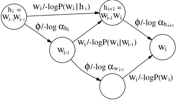
2.1.1 Standard Encoding.For language model encoding, we will differentiate between two classes of transitions:backoff arcs(labeled with aφfor failure, or withusing our new semiring); andn-gram arcs(everything else, labeled with the word whose probabil-ity is assigned). Each state in the automaton represents ann-gram history stringhand eachn-gram arc is weighted with the (negative log) conditional probability of the word wlabeling the arc given the historyh. We assume that, for everyn-gramhwexplicitly represented in the language model, every proper prefix and every proper suffix of that n-gram is also represented in the model. Hence, ifhis a state in the model, thenh0(the suffix ofhof length|h|−1) will also be a state in the model. For a given historyhand n-gram arc labeled with a wordw, the destination of the arc is the state associated with the longest suffix of the stringhwthat is a history in the model. This will depend on the Markov order of then-gram model. For example, consider the trigram model schematic shown in Figure 1, in which only history sequences of length 2 are kept in the model. Thus, from historyhi=wi−2wi−1, the wordwitransitions tohi+1=wi−1wi, which is the

longest suffix ofhiwiin the model.

As detailed in the “otherwise” semantics of Equation (3), backoff arcs transition from statehto a stateh0, typically the suffix ofhof length|h| −1, with weight (−logα_h). We call the destination state a backoff state. This recursive backoff topology terminates at the unigram state (i.e.,h=, no history).

Backoff states of orderkmay be traversed either viaφ-arcs from the higher order n-gram of orderk+1 or via ann-gram arc from a lower ordern-gram of orderk−1. This means that non-gram arc can enter the zeroeth order state (final backoff), and full-order states (history strings of lengthn−1 for a model of ordern) may haven-gram arcs entering from other full-order states as well as from backoff states of history sizen−2.

2.1.2 Exact Encoding of a Backoff Model with Lexicographic Language Model Semiring.For an LM machineMon the tropical semiring with failure transitions, we can simulate

φ-arcs in a standard LM topology by a topologically equivalent machineM0 on the lexicographichT,Tisemiring, whereφhas been replaced with epsilon, as follows. Let siands0ibe equivalent states inMandM0, respectively. For everyn-gram arc with label

wand weightc, source statesi and destination statesj, construct ann-gram arc with

hi =

wi-2wi-1

hi+1=

wi-1wi

wi/-logP(wi|hi)

wi-1 φ/-logαhi

wi φ/-logαhi+1

wi/-logP(wi|wi-1)

φ/-logαwi-1

wi/-logP(wi)

Figure 1

ADDARC(L,s1, Arc(s2,li,lo,w))

1 add arc to Arcs(s1, L) 2 next-state(arc)←s2 3 in-label(arc)←li

4 out-label(arc)←lo

5 weight(arc)←w

CONVERT2LEXLM(L) 1 n← max

sin States(L)length(history(s)) 2 L0←newFST

3 for sin States(L)do 4 add states0to L0

5 if sis Start(L)then If (unique) start state 6 Start(L0)←s0

7 if Final(s, L) =∞then If state not final 8 Final(s0, L0)← h∞,∞i

9 else Final(s0, L0)← h0, Final(s, L)i 10 for arc in Arcs(s, L)do

11 if in-label(arc) =φthen If backoff arc 12 k←length(history(next-state(arc)))

13 ADDARC(L0,s0, Arc(next-state(arc)0,,,hΦ⊗(n−k)_{, weight(arc)i))}

14 else ADDARC(L0,s0, Arc(next-state(arc)0, in-label(arc), out-label(arc),h0, weight(arc)i)) 15 returnL0

Figure 2

Pseudocode for converting ann-gram failure language model into an equivalent lexicographic language model acceptor. The states have an associated history whose length depends on the degree of backoff.

labelw, weighth0,ci, source states0_i, and destination states0_j. The exit cost of each state is constructed as follows. If the state is non-final, the cost ish∞,∞i. Otherwise if it is final with exit costc, it will beh0,ci.

The pseudocode for converting a failure encoded language model into lexico-graphic language model semiring is enumerated in Figure 2 and illustrated in Figure 3. Letnbe the length of the longest history string in the model. For everyφ-arc with (backoff) weightc, source statesi, and destination statesjrepresenting a history of length

k, construct an-arc with source states0_i, destination states0_j, and weight hΦ⊗(n−k),ci, where Φ>0 andΦ⊗(n−k)takesΦ to the (n−k)th power with the⊗operation. In the tropical semiring,⊗is+, soΦ⊗(n−k)=(n−k)Φ. For example, in a trigram model, if we are backing off from a bigram stateh(history length = 1) to a unigram state,n−k=2−

0=2, so we set the backoff weight toh2Φ,−logα_h) for someΦ>0. In the special case where theφ-arc has weight∞, which can happen in some language model topologies, the correspondinghT,Tiweight will beh∞,∞i.

wx xy

y/<0,-logP(y|wx)>

x

ε/<1,-log(α_wx)>

y

ε/<1,-log(α_xy)> y/<0,-logP(y|x)>

ε/<2,-log(α_x)> y/<0,-logP(y)>

Figure 3

An example to illustrate the encoding of lexicographic language model semiring, where we setΦto 1. This is an instance of the general trigram LM depicted in Figure 1 with the sequence wi−2wi−1wi=wxy. The scalar negative log probabilities are transformed from tropical semiring

In order to combine the model with another automaton or transducer, we would need to also convert those models to thehT,Tisemiring. For these automata, we simply use a default transformation such that every transition with weightcis assigned weight

h0,ci. For example, given a word latticeL, we convert the lattice toL0in the lexicographic semiring using this default transformation, and then perform the intersectionL0∩M0. By removing epsilon transitions and determinizing the result, the low cost path for any given string will be retained in the result, which will correspond to the path achieved withφ-arcs. Finally we project the second dimension of thehT,Tiweights to produce a lattice in the tropical semiring, which is equivalent to the result ofL∩M, namely,

C₂(det(eps-rem(L0∩M0)))=L∩M (4)

whereC₂denotes projecting the second-dimension of thehT,Tiweights,det(·) denotes determinization, andeps-rem(·) denotes-removal.

2.2 Proof of Equivalence

We wish to prove that for any machineN, ShortestPath(M0∩N0) passes through the equivalent states inM0to those passed through inMfor ShortestPath(M∩N). Therefore determinization of the resulting intersection after-removal yields the same topology as intersection with the equivalentφmachine. Intuitively, because the first dimension of thehT,Tiweights is 0 forn-gram arcs and>0 for backoff arcs, the shortest path will traverse the fewest possible backoff arcs; further, because higher-order backoff arcs cost less in the first dimension of thehT,Tiweights in M0, the shortest path will include n-gram arcs at their earliest possible point.

We prove this by induction on the state-sequence of the path p/p0 up to a given statesi/s0i in the respective machinesM/M0.

Base case:Ifp/p0is of length 0, and therefore the statessi/s0i are the initial states of the

respective machines, the proposition clearly holds.

Inductive step: Now suppose thatp/p0 visitss0. . .si/s00. . .s0i and we have therefore

reachedsi/s0i in the respective machines. Suppose the cumulated weights ofp/p0 are

WandhΨ,Wi, respectively. We wish to show that whicheversjis next visited onp(i.e.,

the path becomess0. . .sisj), the equivalent states0is visited onp0(i.e., the path becomes

s0₀. . .s0_is0_j).

Letwbe the next symbol to be matched leaving statessiands0i. There are four cases

to consider:

1. There is ann-gram arc leaving statessiands0ilabeled withw, but no

backoff arc leaving the state.

2. There is non-gram arc labeled withwleaving the states, but there is a backoff arc.

3. There is non-gram arc labeled withwand no backoff arc leaving the states.

4. There is both ann-gram arc labeled withwand a backoff arc leaving the states.

will point tosj ands0j, respectively. Case (3) leads to failure of intersection with either

machine. This leaves case (4) to consider. InM, because there is a transition leaving state silabeled withw, the backoff arc, which is a failure transition, cannot be traversed, hence

the destination of then-gram arcsjwill be the next state inp. However, inM0, both the

n-gram transition labeled withwand the backoff transition, now labeled with, can be traversed. What we will now prove is that the shortest path throughM0cannot include the backoff arc in this case.

In order to emit wby taking the backoff arc out of state s0_i, one or more backoff () transitions must be taken, followed by ann-gram arc labeled withw. Letkbe the order of the history represented by state s0_i, hence the cost of the first backoff arc is

h(n−k)Φ,−log(α_s0

i)iin our semiring. If we traversembackoff arcs prior to emitting the w, the first dimension of our accumulated cost will bem(n−k+m−₂1)Φ, based on our algorithm for the construction ofM0given in Section 2.1.2. Lets0_lbe the destination state after traversing mbackoff arcs followed by ann-gram arc labeled with w. Note that, by definition, m≤k, and k−m+1 is the order of state s0_l. Based on the construction algorithm, the states0_l is also reachable by first emittingwfrom states0_i to reach states0_j followed by some number of backoff transitions, as can be seen from the paths between state wi−1 and wi in the trigram model schematic in Figure 1. The order of state s0j

is either k(if k is the highest order in the model) or k+1 (by extending the history of state s0_i by one word). If it is of orderk, then it will require m−1 backoff arcs to reach state s0_l, one fewer than the path to states0_l that begins with a backoff arc, for a total cost of (m−1)(n−k+m−₂1)Φ, which is less than m(n−k+m−₂1)Φ. If state s0_j is of orderk+1, there will bembackoff arcs to reach states0_l, but with a total cost of m(n−(k+1)+m−₂1)Φ =m(n−k+m−₂3)Φ, which is also less than m(n−k+m−₂1)Φ. Hence the states0_lcan always be reached froms0_iwith a lower cost through states0_jthan by first taking the backoff arc from s0_i. Therefore the shortest path onM0must follow s0₀...s0_is0_j.2

This completes the proof.

2.3 Experimental Comparison of,φ, andhT,T iEncoded Language Models

For our experiments we used lattices derived from a very large vocabulary contin-uous speech recognition system, which was built for the 2007 GALE Arabic speech recognition task, and used in the work reported in Lehr and Shafran (2011). The lexicographic semiring was evaluated on the development set (2.6 hours of broadcast news and conversations; 18K words). The 888 word lattices for the development set were generated using a competitive baseline system with acoustic models trained on about 1,000 hours of Arabic broadcast data and a 4-gram language model. The language model consisting of 122Mn-grams was estimated by interpolating 14 components. The vocabulary is relatively large at 737K, and the associated dictionary has only single pronunciations.

The language model was converted to the automaton topology described earlier, using OpenFst (Allauzen et al. 2007), and represented in three ways: (1) as an approxi-mation of a failure machine using epsilons instead of failure arcs; (2) as a correct failure machine; and (3) using the lexicographic construction derived in this article. Note that all of these options are available for representing language models in the OpenGrm library (Roark et al. 2012).

comparable to the state-of-the-art on this task.2 For the shortest paths, the failure and lexicographic machines always produced identical lattices (as determined by FST equivalence); in contrast, 78.6% of the shortest paths from the epsilon approximation are different, at least in terms of weights, from the shortest paths using the failure LM. For full lattices 6.1% of the lexicographic outputs differ from the failure LM outputs, due to small floating point rounding issues; 98.9% of the epsilon approximation outputs differ.3 In terms of size, the failure LM, with 5.7 million arcs, requires 97 Mb. The equiv-alenthT,Ti-lexicographic LM requires 120 Mb, due to the doubling of the size of the weights.4 _{To measure speed, we performed the intersections 1,000 times for each of}

our 888 lattices on a 2993 MHz Intel Xeon CPU, and took the mean times for each of our methods. The 888 lattices were processed with a mean of 1.62 seconds in total (1.8 msec per lattice) using the failure LM; using thehT,Ti-lexicographic LM required 1.8 seconds (2.0 msec per lattice), and is thus about 11% slower. Epsilon approximation, where the failure arcs are approximated with epsilon arcs, took 1.17 seconds (1.3 msec per lattice). The slightly slower speeds for the exact method using the failure LM, and

hT,Tiare due to the overhead of (1) computation of the failure function at runtime for the failure LM, and (2) determinization for thehT,Tirepresentation. After intersection (and determinization, if required), there is no size difference in the lattices resulting from any of the three methods.

In this section we have shown that the failure-arc representation of backoff in a finite-state language model topology can be exactly represented using arcs, and weights in thehT,Tilexicographic semiring.

We turn in the next section to another application of lexicographic semirings, this time involving a novel string semiring as one of the components.

3. Tagging Determinization on Lattices

In many applications of speech and language processing, we generate intermediate results in the form of a lattice to which we apply finite-state operations. For example, we might POS tag the words in an ASR output lattice as an intermediate stage for detecting out-of-vocabulary nouns. This involves composing the lattices with a POS tagger and will result in a weighted transducer that maps from input words to tags.

Suppose we want from that transducer all the recognized word sequences, but for each word sequence just the single-best tagging. One obvious way to do this would be to extract sublattices containing all possible taggings of each word sequence, compute the shortest path of each such sublattice, and unite the results back together. There are various ways this might be accomplished algorithmically, but in general it will be an expensive operation.

With a little thought it will be clear that at an appropriate level of abstraction the problem we have just described involves determinization. That is, the result is deterministic in the sense that for any input, there is a unique path through the

2 The error rate is a couple of points higher than in Lehr and Shafran (2011) because we discarded non-lexical words, which are absent in maximum likelihood estimated language model and are typically augmented to the unigram backoff state with an arbitrary cost, fine-tuned to optimize performance for a given task.

3 The very slight differences in these percentages (less than 3% absolute in all cases) versus those originally reported in Roark, Sproat, and Shafran (2011) are due to small changes in conversion from ARPA format language models to OpenFst encoding in the OpenGrm library (Roark et al. 2012), related to ensuring that, for everyn-gram explicitly included in the model, every proper prefix and proper suffix is also included in the model, something that the ARPA format does not require.

lattice. But one cannot simply apply transducer determinization because, for one reason, any given input may have multiple outputs and thus is non-functional and not even p-subsequential (Mohri 2009).

In this section we describe two methods, both of which make use of novel weight classes consisting of a pair of a tropical weight and a string weight, which allow a solution that involves determinization on anacceptorin that semiring. One, due to Povey et al. (2012), is described in Section 3.1. Our own work, also previously reported in Shafran et al. (2011), is presented in Sections 3.2 and 3.3. In Section 3.4 we compare the approaches for efficiency.

3.1 Povey et al.’s Approach

Povey et al. (2012) define an appropriate pair weight structure such that determinization yields the single-best path for all unique sequences. In their pair weight (T,S),Tis the original (tropical) weight in the lattice, and Sis a form of string weight representing the tags. Using here the more formal ‘·’ to denote concatenation, they define⊕and⊗

operations as:

(w1,w2)⊕(w3,w4)=       

     

(w1,w2) ifw1<w3; else

(w3,w4) ifw1>w3; else

(w1,w2) if|w2|<|w4|; else

(w3,w4) if|w2|>|w4|; else

(w1,w2) ifw2<Lw4; else

(w3,w4)

(w1,w2)⊗(w3,w4)=(w1+w3,w2·w4) (5)

Here |wi| denotes the length of the sequence wi. The ⊕ of two pair weights in this

definition does not necessarily left-divide the weights, so the standard definition of determinization does not work on this semiring. They change the standard determiniza-tion of a lexicographic semiring by defining a new “common divisor” operadeterminiza-tion

for their pair weight. In the standard determinization, ⊕operation finds the common divisor of the weights.

(w1,w2)(w3,w4)=(w1⊕w3,LongestCommonPrefix(w2,w4)) (6)

Povey et al. describe their method in the context of an exact lattice generation task. They create a state-level lattice during ASR decoding and determinize it to retain only the best-scoring path for each word sequence. They invert the state-level lattice, encode it as an acceptor with its input label equal to the input label of lattice (word), and the pair weight equal to the weight and output label of the lattice, and finally determinize the acceptor to get the best state-level alignment for each word sequence.

For efficiency reasons, determinization and epsilon removal (which is optimized for this particular type of weight) are done simultaneously in their method. For the string part, they use a data structure involving a hash table which enables string concatenation in linear time.

3.2 Categorial Semiring

library. To this end, we designed a lexicographic weight pair that incorporates a tropical weight as the first dimension and a novel form of string weight for the second dimen-sion to represent the tags. Note that the standard string weight (e.g., that implemented in the OpenFst library) will not do. In that semiring,w1⊗w2is defined as concatenation;

and w1⊕w2 is defined as the longest common prefix of w1 and w2, which is not in

general equal to eitherw1 or w2. Thus the string weight class does not have the path

property, and hence it cannot be used as an element of a lexicographic semiring tuple. We can solve that problem by havingw1⊕w2 be the lexicographic minimum

(ac-cording to some definition of string ordering) ofw1 andw2, which will guarantee that

the semiring has the path property. But now we need a way to make the semiring weakly divisible, so that when weights are pushed during the determinization operation, the “loser” can be preserved. For a string weight, this can be achieved by recording the division so that a subsequent⊗operation with the appropriate (inverse) string is cancellative. Thus ifx⊕y=y, then there should be az=y\x, such that (x⊕y)⊗z= (x⊕y)⊗y\x=y⊗y\x=x.

A natural model for this iscategorial grammar(Lambek 1958). In categorial gram-mar, there are a set of primitive categories, such asN,V,NP, as well as a set of complex types constructed out of left (\) or right (/) division operators. An expression X\Y denotes a category that, when combined with anXon its left, makes aY. For example, a verb phrase in English could be represented as aNP\S, because when combined with anNPon the left, it makes anS. Similarly, a determiner isNP/N, because it combines with anNon the right to make anNP.

Acategorial semiringcan be defined for both left- and righthand versions. We restrict ourselves in this discussion to the left-categorial semiring, the right-categorial version being equivalently defined. Thus we define theleft-categorialsemiring (Σ∗,⊕,⊗,∞_s,) over strings Σ∗ with and ∞_s as special infinity and null string symbols, respec-tively (as in the normal string semiring). The ⊗ operation accumulates the symbols along a path using standard string concatenation. The⊕operation simply involves a string comparison between the string representations of (possibly accumulated versions of) the output symbols or tags using lexicographic less-than (<_L). The ; operation records the left-division in the same sense as categorial grammar. Finally, we introduce a function REDUCE, which performs reductions on any string, so that for example REDUCE(a·a\b)=b:

w1⊕w2=

w1ifw1<Lw2 w2otherwise

w1⊗w2=REDUCE(w1·w2)

w1;w2=w2\w1 (7)

We further define grouping bracketshandias part of the notation so that, for example, a complex weighta\bcdivided intodisha\bci\d.

Unfortunately, although this definition is close to what we want, it is not a semiring, because with that definition,⊗is not distributive over⊕. As stated in Section 1.1, a semiring must be defined in such a way thatw1⊗(w2⊕w3)=(w1⊗w2)⊕(w1⊗w3).

To see that this is not in general the case with the above definition, letw1=c,w2=c\a

andw3 =b. Using ‘ ’ to indicate concatenation of two weights, and assuming thata<L

b<_Lc, then:

whereas

(c⊗c\a)⊕(c⊗b)=a⊕c b=a (9)

To solve this problem requires modifying our semiring definition slightly to distinguish between the history, denoted as h, and the value, denoted as v. The history records the concatenations involved in creating the particular weight instance, without any concomitant reductions, and the value is the actual value of the weight, including the reductions. We redefine the left categorial semiring as follows:

w1⊕w2=

w1ifh(w1)<Lh(w2) w2otherwise

w1⊗w2=w3, whereh(w3)=h(w1)·h(w2) andv(w3)=REDUCE(h(w3))

w1;w2=w3, whereh(w3)=h(w2)\h(w1) andv(w3)=v(w2)\v(w1) (10)

Note that the history now defines the natural ordering of the semiring. Returning to the earlier problematic case we note that it is still the case thatc⊗(c\a⊕b)=c⊗b=

c b. This is because forc\a⊕b,h(b)<_Lh(c\a), so thatc\a⊕b=b. For (c⊗c\a)⊕(c⊗b), however, we now get the same result. (c⊗b) has both a history and a value of c b. (c⊗c\a), on the other hand, has a value ofaas before, but a history ofc c\a. The sum of these weights is determined by the lexicographic comparisonc b<_Lc c\a, and thus (c⊗c\a)⊕(c⊗b)=c b.

The value of⊗is defined as the reduction of thehistoryof the concatenated weight histories rather than the concatenated weight values, in order to guarantee that ⊗is associative: for semiring⊗ it must be the case thatw1⊗(w2⊗w3)=(w1⊗w2)⊗w3.

Letw1=a,w2 =a\b, andw3 =ha\bi\c. If we compute the values of the multiplications

on the basis of the values of the weights, we have

a⊗(a\b⊗ ha\bi\c)=a⊗c=a c (11)

but

(a⊗a\b)⊗ ha\bi\c=b⊗ ha\bi\c=bha\bi\c (12)

However, the histories in both cases are given as:

a⊗(a\b⊗ ha\bi\c)=a a\b ha\bi\c

=(a⊗a\b)⊗ ha\bi\c (13)

interpretation of this category is something that, when combined with the category VB\JJ NNon the left, makes anNN.

3.3 Implementation of Tagging Determinization Using a Lexicographic Semiring

Having chosen the semirings for the first and second weights in the transformed weighted finite-state automaton, we now need to define a joint semiring over both the weights and specify its operation. For this we return to the lexicographic semiring. Specifically, we define the hT,Ci lexicographic semiring (h< ∪ {∞},Σ∗i,⊕,⊗, ¯0, ¯1) over a tuple of tropical and left-categorial weights, inheriting their corresponding identity elements. The ¯0 and ¯1 elements for the categorial component are defined the same way as in the standard string semiring, namely, respectively, as the infinite string, and as the empty string, discussed previously.

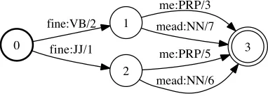
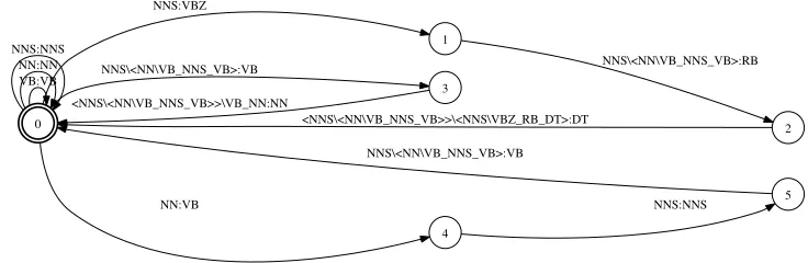
A Sketch of a Proof of Correctness: The correctness of this lexicographic semiring, combined with determinization, for our problem could be shown by tracing the results of operation in a generic determinization algorithm, as in Mohri (2009). Instead, here we provide an intuition using the example in Figure 4. The two input stringsfine me andfine meadshare the prefixfine. In the first case,fineis a verb (VB), whereas in the second it is an adjective (JJ). When two outgoing arcs have the same input symbols, the determinization algorithm chooses the arc with the lowest weight,h1,JJi. For potential future use the other weight h2,VBi is divided by the lowest weight h1,JJi and the result h1,JJ\VBi is saved. (Note that the divide operation for the tropical semiring is arithmetic subtraction.) When processing the next set of arcs, the determinization algorithm will encounter two paths for the inputfine mead. The accumulated weight on the path through nodes 0-2-3 is straightforward and ish1,JJi ⊗ h6,NNi=h7,JJ_NNi. The accumulated weight computed by the determinization algorithm through 0-1-3 consists of three components: the lowest weight forfine, the saved residual, and the arc weight formeadfrom 1-3. Thus, the accumulated weight for 0-1-3 forfine meadis

h1,JJi ⊗ h1,JJ\VBi ⊗ h7,NNi=h9,VB_NNi. From the two possible paths that terminate at node 3 with input stringfine mead, the determinization algorithm will pick one with the lowest accumulated weight,h7,JJ_NNi ⊕ h9,VB_NNi=h7,JJ_NNi, the expected re-sult. Similarly, the determinization algorithm for the inputfine mewill result in picking the weighth5,VB_PRPi. Thus, the determinization algorithm will produce the desired result for both input strings in Figure 4 and this can be shown to be true in general.

After determinization, the output symbols (tags) on the second weight may accu-mulate in certain paths, as in the earlier example. These weights need to be mapped back to associated input symbols (words). This mapping and the complete procedure for

0

1 fine:VB/2

2

fine:JJ/1 3

me:PRP/3

mead:NN/7

me:PRP/5

mead:NN/6

Figure 4

0

1 time:NN/0.25

6 time:NN/0.25

9 time:VB/0.5

12 time:NN/0.25

2 flies:VBZ/1

7 flies:NNS/0.9

10 flies:NNS/0.7

13 flies:NNS/1

3

like:RB/0.9 an:DT/0.8 ₄

5 arrow:NN/0.2

8

like:VB/0.7 _meat:NN/0.5

11

like:VB/0.3 wasps:NNS/1.2

14

like:RB/2.5 an:DT/0.8 ₁₅

arrow:NN/0.2

Figure 5

Sample input lattice.

computing the single-best transduction paths for all unique input sequences for a given WFST (word lattice) using the hT,Ci lexicographic semiring is described in the next few sections. Note that our categorial semiring allows for synchronizing the resulting output labels with their associated input labels, which the Povey et al. (2012) approach in general does not.

3.3.1 Lattice Representation.Consider a lattice transducer where input labels are words (e.g., generated by a speech recognizer), output labels are tags (e.g., generated by a part-of-speech tagger), and weights in the tropical semiring represent negative log probabilities. For example, the toy lattice in Figure 5 has four paths, with two possible tag sequences for the string Time flies like an arrow. In general, for any given word sequence, there may be many paths in the lattice with that word sequence, with different costs corresponding to different ways of deriving that word sequence from the acoustic input, as well as different possible ways of tagging the input.

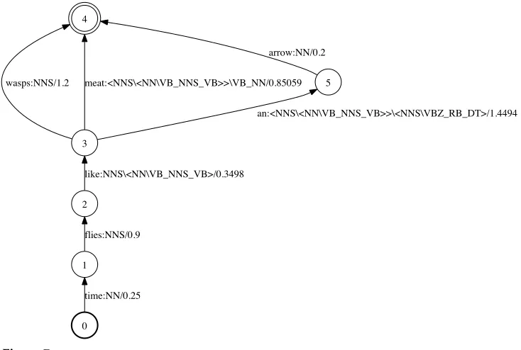
The procedure for removing all but the single best-scoring path for each input word sequence is as follows. We convert the weighted transducer to an equivalent acceptor in thehT,Ci-lexicographic semiring as in the algorithm in Figure 6. This acceptor is then determinized in thehT,Ci-lexicographic semiring, to yield a lattice where each distinct sequence of input-labels (words) corresponds to a single path. The result of converting the lattice in Figure 5 to thehT,Cisemiring, followed by determinization, and conver-sion back to the tropical semiring, is shown in Figure 7. Note now that there are three paths, as desired, and that the tags on several of the paths are complex categorial tags.

We now have an acceptor in the hT,Ci-lexicographic semiring with, in general, complex categorial weights in the second component of the weight pair. It is now necessary to simplify these categorial weight sequences down to sequences of simplex categories, and reconstruct a transducer that maps words to tags with tropical weights. Figure 8 presents the result of such a simplification.

There are two approaches to this, outlined in the next two sections. The first in-volves pushinghT,Ci-lexicographic weights back from the final states, splitting states as needed, and then reconstructing the now simple categorial weights as output labels on the lattice. The latter reconstruction is essentially the inverse of the algorithm in Figure 6. The second approach involves creating a transducer in the tropical semiring with the input labels as words, and the output labels as complex tags. For this approach we need to construct a mapper transducer which, when composed with the lattice, will reconstruct the appropriate sequences of simplex tags.

CONVERT(L) 1 L0←newFST 2 for sin States(L)do 3 add states0to L0

4 if sis Start(L)then If (unique) start state

Start(L0)←s0

5 if Final(s, L) =∞then If state not final

Final(s0, L0)← h∞,∞_si

6 else Final(s0, L0)← hFinal(s, L),i

7 for arc in Arcs(s, L)do

8 ADDARC(L0,s0, Arc(next-state(arc)0, in-label(arc), in-label(arc),

hweight(arc), out-label(arc)i)) 9 returnL0

Figure 6

Pseudocode for converting POS-tagged word lattice into an equivalenthT,Cilexicographic acceptor, with the arc labels corresponding to the input label of the original transducer.

The categorial weights of each arc are split into a prefix and a suffix, according to the SPLITWEIGHTfunction of Figure 9. The prefixes will be pushed towards the initial state, but if there are multiple prefixes associated with arcs leaving the state, then the state will need to be split: Forkdistinct prefixes, kdistinct states are required. The PUSHSPLIT

algorithm in Figure 10 first accumulates the set of distinct prefixes at each state (lines 5–13), as well as storing the vector of arcs leaving the state, which will be subsequently modified. For each prefix, a new state is created (lines 22–25), although the first prefix in the set simply uses the state itself. Note that any categorial weight

0 1

time:NN/0.25 2

flies:NNS/0.9 3

like:NNS\<NN\VB_NNS_VB>/0.3498 4

wasps:NNS/1.2 meat:<NNS\<NN\VB_NNS_VB>>\VB_NN/0.85059 5

an:<NNS\<NN\VB_NNS_VB>>\<NNS\VBZ_RB_DT>/1.4494 arrow:NN/0.2

Figure 7

0

2 time:NN/0.25

1 time:VB/0.25

5 flies:VBZ/0.9

4 flies:NNS/0.9

3 flies:NNS/0.9

6 like:VB/0.3498

8 like:RB/0.3498

7

like:VB/0.3498 ₉

wasps:NNS/1.2 meat:NN/0.85059

10 an:DT/1.4494

arrow:NN/0.2

Figure 8

Final output lattice with the desired three paths.

associated with the final cost yields the first prefix, meaning that it would be assigned the already existing state; hence all newly created states can be non-final. Each state is thus associated with a distinct single prefix, and each must be reachable from the same set of previous states as the original state. Thus, for each new state, any arc that already has the original state as its destination state must be copied, and the new arc assigned the new destination state and weight, depending on the prefix associated with the new state (lines 26–30). The prefix associated with the original state must then be pushed onto the appropriate arcs (line 29). Finally, because all the prefix values have been pushed, each arc from the original state must be updated so that only the suffix value remains in the weight, now leaving the state associated with the original weight’s prefix (lines 31–34).

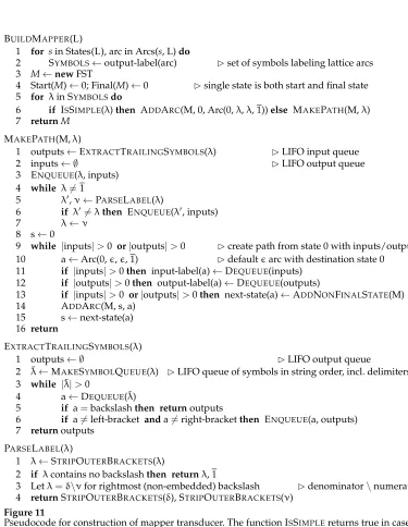
3.3.3 Mapper Approach. In the second approach, we build amapper FST (M) that con-verts sequences of complex tags back to sequences of simple tags. The algorithm for constructing this mapper is given in Figure 11, and an illustration can be found in Fig-ure 12. In essence, sequences of observed complex tags are interpreted and the resulting simplex tags are assigned to the output tape of the transducer. Simplex tags in the lattice are mapped to themselves in the mapper FST (line 6 of the function BUILDMAPPERin Figure 11); complex tags require longer paths, the construction of which is detailed in the MAKEPATHfunction. The complex labels are parsed, and required input and output labels are placed on LIFO queues (lines 3–7). Then a path is created from state 0 in the mapper FST that eventually returns to state 0, labeled with the appropriate input and output sequences (lines 9–15).

Once the mapper FST has been constructed, the determinized transducer is com-posed with the mapper—L0◦M—to yield the desired result, after projecting onto output labels. Note, crucially, that the mapper will in general change the topology of the deter-minized acceptor, splitting states as needed. This can be seen by comparing Figures 7 and 8. Indeed, the mapping approach and PUSHSPLITare completely equivalent, and, as we shall see, have similar time efficiency.

SPLITWEIGHT(w)

1 if w = 0 or w = 1then returnw, w 2 if w is atomicthen return1, w

3 By construction, complex weights must end in an atomic weight, i.e., a simplex tag 4 if w = a\b, where b is atomic either final atomic weight is preceded by a division

5 then returnw, 1

6 let w = a b, where b is atomic or final atomic weight is concatenated to the preceding

7 returna, b

Figure 9

PUSHSPLIT(L)

1 TopologicallySort(L)

2 for s in States(L)do For each s, find all states with outgoing arcs with destination s 3 previous[s]←COMPUTEPREVIOUSSTATES(s, L)

4 for s in Reverse(States(L))do Work on states in reverse topological order 5 prefixes← ∅; arcs← ∅ initialize prefix and arcs vectors

6 if FinalWeight(s)6=0 If non-zero final weight, then: 7 then append Value2(FinalWeight(s)) to prefixes Categorial component of final 8 Value2(FinalWeight(s))←1 weight is a prefix; reset to 1 9 for a in Arcs(s, L)do For all outgoing arcs from s

10 append a to arcs store arc in arcs vector

11 prefix, suffix←SPLITWEIGHT(Value2(Weight(a)))

12 if prefix not in prefixes Store unique prefixes in vector 13 then append prefix to prefixes

14 DeleteArcs(s, L) Will replace with updated arcs later 15 previous-arcs← ∅

16 for previous-s in previous[s]do For all arcs with destination state s 17 for a in Arcs(previous-s, L) such that next-state(a) = sdo

18 a0_←a

19 delete a

20 append<previous-s, a0_{>to previous-arcs}

21 new-states← ∅

22 for prefix in prefixesdo

23 if new-states =∅ first prefix (from FinalWeight if non-zero) uses s 24 then new-states[prefix]←s

25 else new-states[prefix]←ADDNONFINALSTATE(L)

26 for <previous-s, arc>in previous-arcsdo For all arcs with destination s

27 a←arc create new arc

28 next-state(a)←new-states[prefix] update destination 29 Value2(Weight(a))←Value2(Weight(a))⊗prefix push prefix 30 ADDARC(L, previous-s, a)

31 for a in arcsdo

32 prefix, suffix←SPLITWEIGHT(Value2(Weight(a)))

33 Value2(Weight(a))←suffix Categorial component of weight is now just suffix 34 ADDARC(L, new-states[prefix], a) Origin state of arc is based on prefix

35 return

Figure 10

Pseudocode for the PUSHSPLITalgorithm on a latticeLin thehT,Cisemiring. Note that Value2(w) for weightwis the categorial component of the weight. For the SPLITWEIGHT algorithm, see Figure 9.

To understand the semantics of the categorial weights, consider the path that con-tains the wordsflies like meat, which has the categorial tag sequence

NNS NNS\<NN\VB_NNS_VB> <NNS\<NN\VB_NNS_VB>>\VB_NN

in Figure 7. The cancellation, working from right to left, first reduces

<NNS\<NN\VB_NNS_VB>>\VB_NN

with

NNS\<NN\VB_NNS_VB>

yielding

This then is concatenated with the initial simplex category to yield the sequence NNS VB NN. The actual cancellation is performed by the mapper transducer in Figure 12; the cancellation just described can be seen in the path that exits state 0, passes through state 3, and returns to state 0.

The construction in the case of the PUSHSPLIT algorithm is more direct because it operates on the determinized latticebefore it is converted back to the tropical semiring; after which the simplex categories are reconstructed onto the output labels to yield a transducer identical to that in Figure 8.

BUILDMAPPER(L)

1 for sin States(L), arc in Arcs(s, L)do

2 SYMBOLS←output-label(arc) set of symbols labeling lattice arcs 3 M←newFST

4 Start(M)←0; Final(M)←0 single state is both start and final state 5 for λin SYMBOLSdo

6 if ISSIMPLE(λ)then ADDARC(M, 0, Arc(0,λ,λ, 1))else MAKEPATH(M,λ)

7 returnM

MAKEPATH(M,λ)

1 outputs←EXTRACTTRAILINGSYMBOLS(λ) LIFO input queue

2 inputs← ∅ LIFO output queue

3 ENQUEUE(λ, inputs)

4 while λ6=1

5 λ0,ν←PARSELABEL(λ)

6 if λ06=λthen ENQUEUE(λ0, inputs)

7 λ←ν

8 s←0

9 while |inputs|>0 or|outputs|>0 create path from state 0 with inputs/outputs

10 a←Arc(0,,, 1) defaultarc with destination state 0 11 if |inputs|>0then input-label(a)←DEQUEUE(inputs)

12 if |outputs|>0then output-label(a)←DEQUEUE(outputs)

13 if |inputs|>0 or|outputs|>0then next-state(a)←ADDNONFINALSTATE(M) 14 ADDARC(M, s, a)

15 s←next-state(a)

16 return

EXTRACTTRAILINGSYMBOLS(λ)

1 outputs← ∅ LIFO output queue

2 λ¯←MAKESYMBOLQUEUE(λ) LIFO queue of symbols in string order, incl. delimiters 3 while |λ¯|>0

4 a←DEQUEUE( ¯λ)

5 if a=backslashthen returnoutputs

6 if a6=left-bracket anda6=right-bracketthen ENQUEUE(a, outputs)

7 returnoutputs

PARSELABEL(λ)

1 λ←STRIPOUTERBRACKETS(λ)

2 if λcontains no backslashthen returnλ, 1

3 Letλ=δ\νfor rightmost (non-embedded) backslash denominator\numerator

4 returnSTRIPOUTERBRACKETS(δ), STRIPOUTERBRACKETS(ν)

Figure 11

0 VB:VB NN:NN

NNS:NNS 1 NNS:VBZ

3 NNS\<NN\VB_NNS_VB>:VB

4 NN:VB

2 NNS\<NN\VB_NNS_VB>:RB

<NNS\<NN\VB_NNS_VB>>\VB_NN:NN

5 NNS:NNS

<NNS\<NN\VB_NNS_VB>>\<NNS\VBZ_RB_DT>:DT

NNS\<NN\VB_NNS_VB>:VB

Figure 12

After conversion of thehT,Cilattice back to the tropical, this mapper will convert the lattice to its final form.

3.4 Experimental Comparisons Between Povey et al.’s and

hT,Ci-Lexicographic Semirings

3.4.1 POS-Tagging Problem.Our solutions were empirically evaluated on 4,664 lattices from the NIST English CTS RT Dev04 test set. The lattices were generated using a state-of-the-art speech recognizer, similar to Soltau et al. (2005), trained on about 2,000 hours of data, which performed at a word error rate of about 24%. The utterances were decoded in three stages using speaker independent models, vocal-tract length normalized models, and speaker-adapted models. The three sets of models were similar in complexity with 8,000 clustered pentaphone states and 150K Gaussians with diagonal covariances.

The lattices from the recognizer were tagged using a weighted finite state tagger. The tagger was trained on the Switchboard portion of the Penn Treebank (Marcus, Santorini, and Marcinkiewicz 1993). Treebank tokenization is different from the recog-nizer tokenization in some instances, such as for contractions (“don’t” becomes “do n’t”) or possessives (“aaron’s” becomes “aaron ’s”). Further, many of the words in the recognizer vocabulary of 93k words are unobserved in tagger training, and are mapped to an OOV token “hunki”. Words in the treebank not in the recognizer vocabulary are also mapped to “hunki”, thus providing probability mass for that token in the tagger. A tokenization transducerT was created to map from recognizer vocabulary to tagger vocabulary.

Two POS-tagging models were trained: a first-order and a third-order hidden Markov model (HMM), estimated and encoded in tagging transducersP. In the first-order HMM model, the transition probability is conditioned on the previous word’s tag, whereas in the third-order model the transition probability is conditioned on the previous three words’ tags. The transition probabilities are smoothed using Witten-Bell smoothing, and backoff smoothing is achieved using failure transitions. For each word in the tagger input vocabulary, only POS-tags observed with each word are allowed for that word; that is, emission probability is not smoothed and is zero for unobserved tag/word pairs. For a given word latticeL, it is first composed with the tokenizerT, then with the POS taggerP to produce a transducer with original lattice word strings on the input side and tag strings on the output side.

Huang, and Harper (2010) reported accuracy of 92.4% for an HMM tagger on this task (though for a different validation set). Both models likely suffer from using a single “hunki” category, which is relatively coarse and does not capture informative suffix and prefix features that are common in such models for tagging OOVs. For the purposes of this article, these models serve to demonstrate the utility of the new lexicographic semiring using realistic models. A similar WFST topology can be used for discrimina-tively trained models using richer feature sets, which would potentially achieve higher accuracy on the task.

The tagged lattices, obtained from composing the ASR lattice with the POS tag-ger, were then converted tohT,Ci-lexicographic semiring, determinized in this lexico-graphic semiring, and then converted back using the mapper transducer as discussed in Section 3.3.1. Note that the computational cost of this conversion is proportional to the number of arcs in the lattice and hence is significantly lower than the overhead incurred in the conventional approach of extracting all unique paths in the lattice and converting the paths back to a lattice after tagging.

The results of this operation were compared with the method of taking the 1,000 best paths through the original lattice, and removing any path where the path’s word sequence had been seen in a lower-cost path. This generally resulted in a rank-ordered set of paths withn<1, 000 members.

In all cases then-best paths produced by the method proposed in this article were identical to the n-best paths produced by the method just described. The only differ-ences were due to minor floating-point number differdiffer-ences (expected due to weight-pushing in determinization), and cases where equivalent weighted paths were output in different orders.

3.4.2 Results. Despite large overall commonalities between Povey et al.’s approach (henceforth Povey), and hT,Ci lexicographic approaches (henceforth TC), there are some interesting differences between the two. One difference is that the highly struc-tured categorial weights used in TC are more complex than the string weight used in Povey. Another important difference in the approaches is thesynchronization issue. In TC, the original input symbols are synchronized with determinized output symbols, whereas in Povey they are not. TC uses the semantics of the categorial grammar to keep the history of the operations while determinizing a lattice, whereas Povey lacks this semantics. Although POS-tagging is a task that by definition has one tag per input token, many other tasks of interest (e.g., finding the most likely pronunciation or state sequence) will have a variable number of output labels per token, making syn-chronization in the absence of such semantics more difficult. Hence, these differences may affect time and space complexity, feasibility, and ease of use of the approaches in various tasks.

In this section, we compare the efficiency of the two approaches under the same situations on the same data. We ran the experiments detailed in Section 3.4.1 in three conditions: Povey in the Kaldi toolkit (Povey et al. 2011) (with specialized determiniza-tion); and both Povey and TC in the OpenFST library (with general determinization). This allows us to tease apart the impact of the differences in the approaches that are due to the specialized determinization versus differences in the weight definitions. There would be nothing in principle to prevent the simultaneous epsilon removal being implemented in OpenFst for use with general determinization inhT,Cilexicographic semiring, although this is not the focus of this article.

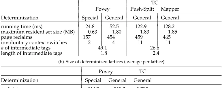
Table 1

For first-order HMM tagger, comparison of the two approaches for extracting the best and only the best POS for all the word sequences in the test lattice. The approach by Povey et al. as implemented in Kaldi using a specialized determinization and our re-implementation in OpenFST with general determinization.

(a) Time, memory usage, disk space and intermediate tags (average per lattice).

TC

Povey Push-Split Mapper

Determinization Special General General General

running time (ms) 24.8 52.5 122.9 128.2

maximum resident set size (MB) 0.63 1.80 1.83 1.85

page reclaims 157 454 459 465

involuntary context switches 2 4 11 11

# of intermediate tags 49.1 26.6

length of intermediate tags 1.8 2.4

(b) Size of determinized lattices (average per lattice).

Povey TC

Determinization Special General General

# of states 344.7 768.2 187.5

# of transitions 565.5 1,295.6 433.5

# final states 7.6 7.6 7.7

# of input epsilons 190.1 602.6 16.7

# of output epsilons 91.7 299.2 0

# size of determinized lattice (KB) 15.1 31.4 11.6

using the first-order HMM tagger, and Tables 2(a), and 2(b) show those results for the third-order HMM tagger.

From Table 1(a) we see that Povey is faster and demands less memory compared with TC. However, results using Povey with general determinization show that the memory demands between the two approaches are similar in the absence of the spe-cialized determinization. We also see that the average number of intermediate tags produced during determinization in Povey is larger, whereas the average length of intermediate tags is smaller, than those in TC. This is due to the fact that the categorial semiring keeps a complete history of operations by appending complex tags. We do not perform any special string compression on these tags, which may yield performance improvements (particularly with the larger POS-tagging model, as demonstrated in Table 2).

We compared the approach of using the mapper with that of the PUSHSPLIT al-gorithm in TC. The outputs were equivalent in both cases and the time and space complexities were comparable. The PUSHSPLIT algorithm was slightly more efficient

than the mapper approach, although the difference is not significant.

As Tables 2(a) and 2(b) show, time and space efficiencies in tagging using the third-order HMM tagger follow the same pattern as those using the first-third-order HMM tagger, although the differences are more pronounced than in the former. We report these results on a subset of 4,000 out of 4,664 test lattices, chosen based on input lattice size so as to avoid cases of very high intermediate memory usage in general determinization. This high intermediate memory usage does argue for the specialized determinization, and was the rationale for that algorithm in Povey et al. (2012). The non-optimized string representation within the categorial semiring makes this even more of an issue for TC than Povey. Again, though, the size of the resulting lattice is much more compact when using the lexicographichT,Cisemiring. We leave investigation of an optimized string representation, such as storing thehistoryonly if it is different from thevalue, using the hash table data structure, or memory caching, to future work.

4. Combining the Semirings

In this article, we have described two lexicographic semirings, each consisting of a weight pair. Suppose one wished to combine these two in a system that tags a lattice, and then selects the single best tagging for each word sequence. An obvious way to do this would be to implement a two-stage process. Apply then-gram Markov model of the tagger with the backoff strategy implemented using the paired tropical semiring in Section 2 with tags as acceptor labels. Then, convert the resulting transducer into the lexicographichT,Cisemiring with words as acceptor labels and determinize to obtain the correct results.

Table 2

For third-order HMM tagger, comparison of the two approaches for extracting the best and only the best POS for all the word sequences in the test lattice. The approach by Povey et al. as implemented in Kaldi using a specialized determinization and our re-implementation in OpenFST with general determinization.

(a) Time, memory usage, disk space, and intermediate tags (average per lattice)

TC

Povey Push-Split Mapper

Determinization Special General General General

running time (sec) 2.9 9.6 49.9 50.7

maximum resident set size (MB) 28.0 62.8 240.9 241.1 page reclaims 7,890.9 16,589.9 62,963.7 63,002.8 involuntary context switches 270.1 895 4,985.4 4,915.2

# of intermediate tags 131.6 70.2

length of intermediate tags 3.1 9.3

(b) Size of determinized lattices (average per lattice)

Povey TC

Determinization Special General General

# of states 4,946.2 19,824.9 2,244.0

# of transitions 6,152.3 25,307.7 4,002.8

# final states 153.1 154.0 174.9

Because the lexicographic semiring is extensible, one might also think of combining the two semirings into a singlehT,T,Cilexicographictriplewhere, for example, the first dimension is the failure arc cost, the second dimension holds the tag cost (n-gram transition costs of tags and the cost of observing the word given the tag), and the third dimension holds the tags represented in the categorial semiring. One might then compose the tagging model with the lattice, and then determinize in one step in the triple semiring.

Although this works in the sense that it is technically possible to construct this semiring and determinize in it, it yields the wrong results. The reason for this is that the lexicographic semirings for the two tasks (the tagging task and the subsequent determinization of the tagged lattice) involve determinization with respect to different labels. In the first task, the backoff models are defined with respect to the Markov chain orn-grams of the tags and the labels on the resulting acceptor are tags. In the second task, the determinization needs to be performed with respect to the word labels to obtain unique tags for all word sequences. A cross product of the two types of labels would not accomplish the task either, because the determinization would then produce unique paths for all word and tag combinations, and not the best tag sequences for all word sequences. There is no obvious or easy way to determinize with respect to both sets of labels simultaneously.

We can illustrate this problem with an example, which is also useful for clearly understanding how each of the semirings functions. The simple example involves a cost-free word lattice consisting of two pathsa a and b a, in a scenario where word acan take two possible tagsA orB. We will assign variables to model costs, so that we can illustrate the range of scenarios where the use of the triple semiring will yield an incorrrect answer, and why. Letc(a:A) be the cost of the tagAwith worda, which in our HMM POS tagger is –log P(a|A). Letg(x,y) be the cost in the grammar (tag sequence model) of transitioning from statexto stateyin the model. See Figure 13 for our exampleL,T,L◦T, andG. All costs in the example are in thehT,Tisemiring for ease of explication; the first dimension of the cost is zero except for backoff arcs inG.

In Figure 14 we show the result ofL◦T◦Gboth after simple composition and after epsilon removal and conversion from a transducer in thehT,Tisemiring to an acceptor in thehhT,Ti,Cisemiring. In the second and third WFSTs, we highlight the paths that have zero cost in the first dimension of that semiring, which are the only paths that can result from determinization (whatever the model costs). These paths only include tag B for the initial instance of symbol a. However, if g(0, 2)+c(a:A)+g(2, 3)+c(a:A)+

g(3, 3)<c(a:B)+g(0, 1)+c(a:A)+g(1, 3), then the tag sequence a:A a:A would have lower (second dimension) cost than a:B a:A, despite having taken a backoff arc. Because using a backoff arc is the only way to produce the tag sequenceA A, then that path should be the result. In order to get the correct result, one must first determinize with x:Y labels as unit (using fstencode) in thehT,Tisemiring; then project into thehT,Ci

semiring and determinize again.

5. Conclusions

(a)L (b)T

(c)L◦T

(d)L◦G

Figure 13

Input unweighted latticeLand tag mapper transducerTinhT,Tisemiring, wherec(x:Y) is the cost of wordxwith tagY. When composed,L◦Tyields a lattice of word:tag sequences.Gis a tag language model, which encodes the smoothed transition probabilities of the HMM tagger. represents backoff transitions; andg(x,y) gives the cost of transitioning from statexto stateyin the model. Again, costs are in thehT,Tisemiring, so that backoff transitions have a cost of 1 in the first dimension.

for example, precomposing the language model with a lexicon and a context model in a CLG model of speech recognition (Mohri, Pereira, and Riley 2002).

The second application was of a hT,Ci lexicographic semiring to the problem of determinizing a tagged word lattice so that each word sequence has the single best tag sequence. This was accomplished by encoding the tags as the second dimension of the hT,Ci semiring, then determinizing the resulting acceptor. Finally we map the second dimension categorial weights back as output labels. This latter stage generally requires that we push complex categorial weights back to reconstruct a sequence of simplex categories, an operation that can be performed in two distinct and equally efficient ways. As part of this work we developed a novel string semiring, the categorial semiring, which we have described in detail for the first time here.

For both of these applications, the lexicographic semiring solution was shown to be competitive in terms of efficiency with alternative approaches.