Abstract— Spectral unmixing of hyperspectral images are based on the knowledge of a set of unknown endmembers. Unique characteristics of hyperspectral dataset enable different processing problems to be resolved using robust mathematical logic such as image classification. Consequently, pixel purity index is used to find endmembers from Washington DC mall hyperspectral image dataset. The generalized reduced gradient algorithm is used to estimate fractional abundances in the hyperspectral image dataset. The WEKA data mining tool is selected to construct random forests and neural networks classifiers from the set of fractional abundances. The performances of these classifiers are experimentally compared for hyperspectral data land cover classification. Results show that random forests give better classification accuracy when compared to neural networks. The study proffers solution to the problem associated with land cover classification by exploring generalized reduced gradient approach with learning classifiers to improve overall classification accuracy. The classification accuracy comparison of classifiers is important for decision maker to consider tradeoffs in accuracy and complexity of methods.
Index Terms— Generalized reduced gradient, hyperspectral image, land cover classification, classifiers.
I. INTRODUCTION
he advancement in remote sensing technology has brought about new perspectives into image processing. The image objects are generally entrenched in a single pixel and hence cannot be detected spatially [1]. The traditional spatial based image processing techniques therefore, cannot be used. The importance of image processing that affords abundant data to be interpreted into useful information is crucial in image classification [2]. The preprocessing of remote sensing images before features extraction is important to remove noise and increase the ability to interpret image data more accurately. All generated images after preprocessing procedure must be as if they were obtained from the same sensor [3].
Hyperspectral instruments developed through remote
Manuscript received July 22, 2012; revised August 08, 2012. This work was supported by University of Witwatersrand, South Africa. University of Johannesburg, South Africa and Tshwane University of Technology, South Africa.
B. T. Abe, School of Electrical and Information Engineering, University of the Witwatersrand, Johannesburg. South Africa. Tshwane University of Technology, South Africa. (Corresponding author: +27761304108; e-mail: [email protected]).
O. O. Olugbara is with the Department of Information Technology, Durban University of Technology, Durban, South Africa (e-mail: [email protected]).
T. Marwala is the Dean of the Faculty of Engineering and the Built Environment, University of Johannesburg, South Africa. (e-mail: [email protected]).
sensing technology are capable of collecting hundreds of images corresponding to wavelength channels, for the same area on earth surface [4]. Hyperspectral images provide abundant spectral information to identify and differentiate between spectrally similar materials. The advantage of using hyperspectral sensors is the ability to provide a high-resolution reflectance spectrum for each pixel in the image [5]. Hyperspectral image data has found applications in areas such as mineral exploration, urban processes, agriculture, risk prevention, land cover mapping, surveillance, resource management, tracking wildfires, detecting biological threats and chemical contamination [6]-[7]. As a result, researchers have developed interest in the mathematical analysis of hyperspectral images [8]-[9].
The ability to obtain useful information from hyperspectral image data has stimulated researchers to use data mining methods to identify valid, novel, potentially useful and ultimately understandable patterns in data [3]. In remote sensing technology, there are varieties of earth objects present in the direct view of sensors because of the complexity of target objects and the limited spatial resolution of remote sensors. The information available in a certain pixels of a remote sensing image is a mixture of information on various ground objects, resulting into mixed pixels [4], [8]-[10]. The presence of mixed pixels has significant effects on some practical applications of remote sensing images such as information extraction, image classification and object detection. It is therefore, an important task in remote sensing study to discover objects and corresponding quantity present in the mixed pixel. This has led to the invention of hyperspectral remote sensing techniques to proffer solutions to the mixed pixel problem in remotely sensed imagery.
This work considers the problem of land cover classification of hyperspectral images by using a linear spectral mixture analysis technique, which is a commonly accepted approach to mixed-pixel classification. Land cover refers to the physical surface of the earth, including various combinations of vegetation types, soils, exposed rocks, water bodies and anthropogenic elements, such as agriculture and built environments [8], [11]. Our objectives are to (i) identify a collection of spectrally pure constituent spectral, which are referred to as the endmembers [12]-[13]. Thereafter, we express the measured spectrum of each mixed pixel as a linear combination of endmembers weighted by fractional abundances that indicate the proportion of each endmember present in the pixel [8], [13], (ii) explore Generalized Reduced Gradient (GRG) optimization algorithm to estimate the fractional abundance in the dataset thereby obtaining the numeric values for land cover
Hyperspectral Image Classification using
Random Forests and Neural Networks
B. T. Abe, O. O. Olugbara and
T. Marwala
the performance of random forests and neural networks classifiers to examine the suitability of GRG algorithm for solving land cover classification problem. The application of machine learning techniques such as random forests and neural networks is usually to predict land cover of un-sampled map units that help to retrieve important information from the scene. This work establishes that in comparison, though the classifiers’ performances are remarkable, random forests give better classification accuracy when compared to neural networks.
II. PROBLEM STATEMENT
The task of land cover classification can be formulated as a linear spectral unmixing problem. The linear spectral unmixing is a sub-pixel classification process that decomposes mixed pixels and determines the combination of fractional abundances. Based upon the linear unmixing model assumptions, each pixel at spatial coordinate (l,p) for a particular band in a remotely sensed hyperspectral image (I) having M number of bands can be formally expressed as [8], [10]: ) , ( ). , ( ) , ( 1 p l n e p l a p l x k z k k
(1) The component x(l,p) is the measured reflectance value at the spectral coordinate (l, p),e
kis the spectral response of the kth endmember, ak(l,p) is fractional abundance of the kth
endmember, n(l,p) denotes the spectral band error and z is the total number of endmembers. For linear spectral mixture analysis, each image pixel is a mixture of various endmembers and the spectrum recorded by the sensor is a linear combination of endmembers spectral [16].
Eq. (1) operates under two physical constraints on fractional abundances to account for the full composition of a mixed pixel [8], [12]. These are (i) Nonnegativity constraint, all abundances should be no negative, that is
l p k kak , 0, 1,2,..., (2)
(ii) The abundances sum to one constraint, ) , ( 1 p l a z k k
= 1 (3) The endmembers ek,k1,2,...,z can be extracted from the image (I) by using a certain algorithm such as Pixel Purity Index (PPI) and Automated Morphological Endmember Extraction (AMEE) [8], [12]-[13] before the equation can be solved for a set of fractional abundances. Extant works on linear spectral unmixing problem [8], [9]-[10] have explored the least square method to estimate a set of fractional abundances as follows.
) , ( ) ( ) ,
(l p e e 1e xl p
aLSU T T (4) Eq. 4 can only satisfy the sum to unity of abundances, but the non-negativity of fractional abundances cannot always be guaranteed. The results obtained by the least square method therefore, are generally not optimal in terms of material quantification [8], [12].
In order to find a set of fractional abundances that simultaneously satisfy these two constraints, the following fully constraint linear spectral unmixing GRG optimization
problem formulation has to be solved to minimize the spectral band error n(l,p).
Minimize: )} ). , ( ) , ( ( ) ). , ( ) , ( {( ) , ( e p l a p l x e p l a p l x p l a T
(5)
Subject to
z kk l p
a p l a
1
1 (, )| (, ) 1 0 (6)
} 1 ) , ( 0 | ) , ( {
2
a l p ak l p (7)
In Equation (5), the expression (X)T represents the transpose vector of the vector (X). To solve Equations (5-7) by applying GRG algorithm [14]-[15], to obtain an estimate of a set of fractional abundances, the PPI algorithm is first applied to extract endmembers from the hyperspectral image. The PPI method efficiently handles hyperspectral imagery as it provides a convenient and physically motivated decomposition of an image in terms of a relatively few components [17]. After a set of endmembers
e
{
e
k}
zk1 is determined, the corresponding fractional abundancesz k k l p
a p l
a(, ){ (, )}1 in a certain pixel vector x(l,p) on the image I is estimated by using the GRG algorithm.
III. DESIGN METHODOLOGY
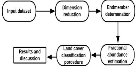
The design methodology of the study entails arrangement of steps that the input hyperspectral image undergoes for its land covers to be classified into one of the desired multiple classes. The input data has to be taken through four steps to obtain the desired classification result. Figure 1 shows the block diagram of the land cover classification process implemented in this study.
Land cover classification porcedure Fractional abundance estimation Endmember determination Dimension reduction Results and discussion Input dataset
Fig 1:Hyperspectral image classification procedure
Before discussing the vital steps used in our design methodology, the input dataset is first introduced.
A. Dataset
[image:2.595.310.539.443.555.2]Fig 2: Hyperspectral image of Washington D. C. mall [18]. Accompany the dataset is a copy of the file labeled dctest.project, which describes the land cover types (also refer to as class labels) used for the experimental procedure. B. Image Dimension Reduction
Dimension reduction as applied to hyperspectral image aims at reducing the number of spectral bands in the image. This is done to map the data into lower dimension from higher dimension at the same time preserve the main features of the original data. The process is carried out to reduce the time used during the processing of the hyperspectral data. The algorithm does not generate an image different from the original image. Instead, it is designed to reduce error by finding minimum representation of the original image that adequately keeps the original information for successful unmixing in the lower dimension [19]. Among various algorithms normally used for dimension reduction are; Principal Component Analysis (PCA) and Maximum Noise Fraction (MNF) transform. The aim is to ease computational complexity and for compact information in transformed components. MNF is used in this study because it is more effective than PCA [20].
C. Endmember Determination
An endmember is known as a spectrally pure pixel that portrays various mixed pixel in an image [21]. The method of feature selection involves identifying the most discriminative measurements out of a set of D potentially useful measurements, where d ≤ D. Endmember extraction has been widely used in hyperspectral image analysis due to significantly improved spatial and spectral resolution provided by hyperspectral imaging sensor also known as imaging spectrometry [20]. Identification of image endmember is a crucial task in hyperspectral data exploitation, especially classification [13]. After endmembers selection, various methods can be used to construct their special distribution, associations and fractional abundances. For real hyperspectral data, various algorithms have been developed to execute the task of locating appropriate endmembers. These include Pixel Purity Index (PPI), N-FINDR and Automatic Morphological Endmember Extraction (AMEE) [20].
This study applies the PPI algorithm [7], [22]-[23], which is available in the Environment for Visualizing Images (ENVI) to determine endmembers from the hyperspectral image. The choice of the algorithm is motivated by its publicity in ITTVIS (http://www.ittvis.com/) ENVI software that was originally developed by Analytical Imaging and Geophysics (AIG) [24]. PPI generates a large number of n- Dimensional vectors called “skewer” [7] [22], through the dataset. N-FINDR fully automated method locates the set of pixels with the largest possible volume by “inflating” a simplex within the image data [21], [25]. In order to
generate the endmembers from the data, “noise whitening” and dimensionality reduction are performed using MNF transform [21], [22]. Then pixel purity score is obtained in the image cube by producing lines in the n-dimension space containing the MNF-transformed data. The spectral points are projected on the lines and the points at the extremes of each line are counted. Bright pixels in the PPI image generally are image endmembers. The highest-valued of these pixels are input into the n-dimensional visualizer for the clustering process that develops individual endmember spectral.
D. Fractional Abundance Estimation
After determining the endmembers using PPI procedure, per pixel fractional abundances of various materials is estimated using GRG optimization method. This study presents six endmember models to characterize the land cover structure which are; Roofs, Street, Path, Grass, Trees, Water and Shadow. Normalized numerical values of the fractional abundant generated were calculated from the spectral signatures of the land cover label signatures. The values obtained were used to train the random forests and neural networks classifiers for land cover classification.
E. Land Cover Classification
Random Forests (RF) and Neural Networks (NN) classifiers are experimentally compared to examine their performances in the field of land cover classification. The WEKA [26] data mining software is selected as a tool to build the classifiers from a training dataset of 3355 instances and 191 band features.
The RF ensemble classifier builds several decision trees randomly as proposed [27] for classification of multisource remote sensing, geographic data and hyperspectral imaging. Various ensemble classification methods have been proposed in recent times and they have been proven to considerably improve classification accuracy. The most famous and widely used ensemble methods are boosting and bagging [27]. The boosting method is based on sample re-weighting technique, but a bagging method uses bootstrapping. RF classifier uses bagging or bootstrap aggregating to yield an ensemble of classification and regression trees. The method works by searching only a random subset of the features for a split at each node to minimize the correlation between the classifiers in the ensemble. The method selects a set of features randomly and creates an algorithm with a bootstrapped sample of the training data [27]. This method provides a potential benefit that it is insensitive to noise or overtraining because resampling is independent of the weighting scheme employed. For our experiment, 10 trees were constructed. Out of bag error was 0.0605 while considering 192 random features.
arbitrary accuracy [28]. Furthermore, they are capable of estimating the posterior capability that provides the basis for creating classification rule and carrying out statistical analysis [28]. Various NN models are available for classification purposes [28], but this paper focuses on MultiLayer Perceptron (MLP) that uses back propagation scheme to classify instances. The nodes in the networks are all sigmoid.
IV. RESULTS AND DISCUSSION
This section presents the results and discussion of our experiment for endmember determination and classification accuracy of the classifiers investigated.
A.Result of Endmember Determination
The first experiment performed aimed to obtain endmembers from image dataset using the ENVI software application. The MNF transformation of input hyperspectral image was performed for dimension reduction. The next stage of the endmember determination is to select a set of endmembers by applying the PPI algorithm on the extracted Region of Interest (ROI) pixels. Figure 3 shows this result, wherein the extreme pixels corresponding to the endmembers in each projection are recorded and total number of times each pixel is marked as extreme is noted. A threshold value of 1 is used to define how many pixels are marked as extreme at the ends of the projected vector.
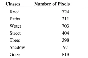
[image:4.595.318.536.45.474.2]Fig 3: Purest pixels occur at edges of the projected vector Table I displays the land cover classes and the number of pixels extracted from the original image based on the ROI. The values of these pixels are input into the ENVI visualizer for the clustering process that develops individual endmember spectral. The pixels extraction mechanism enables the image spectral to accurately account for any errors in atmospheric correction.
TABLEI: NUMBER OF PIXELS EXTRACTED FROM ROI
Classes Number of Pixels
Roof 724
Paths 211
Water 703
Street 404
Trees 398
Shadow 97
Grass 818
The estimated number of spectral endmembers and their corresponding spectral signatures are obtained using ENVI visualizer. Figure 4 shows the generated six fractional endmembers of the image from the PPI method.
Endmember 1
Endmember 2
Endmember 3
Endmember 4
Endmember 5
[image:4.595.124.215.393.482.2]Endmember 6
Fig 4: Fraction images for each endmember
At the completion of specified iterations, a PPI image is created in which the value of each pixel corresponds to the number of times that a pixel was recorded as extreme. The bright pixels in the PPI image are generally the image endmembers to characterize the land cover structure. B.Result of Land Cover Classification
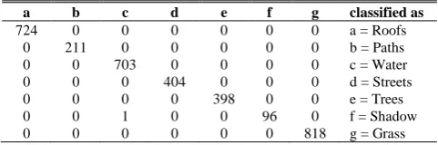
RF and NN classifiers are evaluated using the error confusion matrix method, which is a representation of the entire classification result. According to [29], the error confusion matrix can be used to compute the overall accuracy and the individual class label accuracy. The error confusion matrix is a widely accepted method to report error of raster data and to assess the classification accuracy of a classifier. The matrix expresses the number of sample units allocated to each land cover type as compared to the reference data. The diagonal of the matrix designates agreement between the reference data and the interpreted land cover types [30].
[image:4.595.94.242.602.700.2]is misclassified while shadow has one of the pixels’ members misclassified.
TABLE II: RANDOM FORESTS ERROR CONFUSION MATRIX
a b c d e f g classified as
724 0 0 0 0 0 0 a = Roofs
0 211 0 0 0 0 0 b = Paths
0 0 703 0 0 0 0 c = Water
0 0 0 404 0 0 0 d = Streets
0 0 0 0 398 0 0 e = Trees
0 0 1 0 0 96 0 f = Shadow
0 0 0 0 0 0 818 g = Grass
Table III records the result of the error confusion matrix for the performance of NN. From the table, it can be observed that roofs and grass are 100% classified while other land cover classes have some of their pixels misclassified.
TABLEIII:NEURALNETWORKS ERROR CONFUSION MATRIX
a b c d e f g classified as
724 0 0 0 0 0 0 a = Roofs
1 210 0 0 0 0 0 b = Paths
1 0 699 0 0 3 0 c = Water
1 0 2 401 0 0 0 d = Streets
0 0 0 0 398 0 0 e = Trees
0 0 17 0 0 80 0 f = Shadow
0 0 0 0 0 0 818 g = Grass
Generally, the two classifiers performed excellently well. Considering individual class label, RF produces a higher level of classification accuracy per class label as compared to the NN. The entire accuracy assessment procedure is that the error confusion matrix must be a representative of the entire area mapped from the remotely sensed data [31]-[32]. The overall accuracy for correctly classified instances, incorrectly classified instances, unclassified instances and the Kappa statistic are identified from the error confusion matrices [30]-[33].
If all the non-major diagonal elements of the error confusion matrix are zero, then it means no area in the map has been misclassified and the map accuracy is 100 percent. Otherwise there are certain percentages of misclassified instances [33]. In our experiment, RF as compared to NN has only 1 instance misclassified, while NN has 25 instances misclassified.
The Kappa coefficient of agreement is a measure of how well the accuracy of the classifier compares with the reference or ground truth data [33]. It ranges from 0 to 1, with 0 implying no agreement between the classified land cover and ground truth and 1 indicates complete agreement. Table IV shows the result of error, Kappa statistics and overall accuracy classification.
TABLEIV: CLASSIFICATION ACCURACY
C CCI ICI UI KS MAE RMSE RAE (%)
RRSE (%)
Accuracy (%) RF 3354 1 0 0.9996 0.0015 0.0176 0.6568 5.1615 99.9702
NN 3330 25 0 0.9909 0.003 0.0379 1.2835 11.1095 99.2548
Where: C– Classifier, CCI – Correctly Classified Instances, ICI– Incorrectly Classified Instances, UI – Unclassified Instances, KS – Kappa Statistic, MAE – Mean Absolute Error, RSE – Root Mean Squared error, RAE – Relative Absolute Error, RRSE – Root Relative Squared Error
According to this result, there are no unclassified instances during the RF and NN classification procedures and the overall classification accuracies of the classifiers are seen to be comparable. It can be deduced from the predictions that RF outperformed NN. In addition, RF is more computational effective as compared to NN.
V. CONCLUSION
This study aimed to establish performance comparison between RF and NN classifiers for land cover classification. The performance assessment was done, giving overall accuracy and error confusion matrix. Experimental results demonstrate that the generation of RF and NN based land cover classification systems significantly improve overall accuracy. As a result, the classifiers can significantly contribute to land cover classification system as a source of analysis and increase its accuracy. The comparability and high accuracy performance of RF and NN indicates that the GRG method introduced in this study is effective for solving a linear spectral unmixing problem of land cover classification.
REFERENCES
[1] C. I. Chang and D. C. Heinz, “Constrained subpixel target detection for remotely sensed imagery,” IEEE Trans. Geosci. Remote Sens., vol. 38, no. 3, May 2000, pp. 1144–1159.
[2] H. Liu, Y. Fan, X. Deng and S. Ji, "Parallel Processing Architecture of Remotely Sensed Image Processing System Based on Cluster," Image and Signal Processing, 2009, CISP '09. 2nd International Congress on, 2009, pp.1-4.
[3] Y. Xie, Z. Sha and M. Yu, “Remote sensing imagery in vegetation mapping: a review”, Journal of Plant Ecology, 2008, 1, pp. 9–23. [4] A. Plaza, P. Martínez, J. Plaza, and R. Pérez, “Spectral analysis of
hyperspectral image data,” Advances in Technique for Analysis of Remotely Sensed Data, IEEE Workshop, 2003, pp. 298 – 307. [5] M. A. Karaska, R. L. Hugenin, J. L. Beacham, M. Wang, J. R. Jenson
and R.S. Kaufman, “AVIRIS measurements of chlorophyll, suspended minerals, dissolved organic carbon, and turbidity in the Neuse Rivver, North Calina,” Photogrammetric Engineering and Remote Sensing, vol.70, no. 1, 2004, pp. 125-133.
[6] J.M. Ellis, “Searching for oil seeps and oil-impacted soil with hyperspectral imagery,” Earth Observation Magazine, 2001, pp. 25-28.
[7] F.M. Lacar, M.M. Lewis and I.T. Grierson, "Use of hyperspectral imagery for mapping grape varieties in the Barossa Valley, South Australia," Geoscience and Remote Sensing Symposium, IGARSS '01. IEEE 2001 International, 2001, vol. 6, pp. 2875-2877.
[8] S. Sanchez, G. Martin, A. Plaza, and C. Chang, “GPU implementation of fully constrained linear spectral unmixing for remotely sensed hyperspectral data exploitation”, Proceedings SPIE Satellite Data Compression, Communications, and Processing VI, 2010, 7810, pp. 78100G-1 – 78100G-11.
[9] M-D. Iordache, J. M. Bioucas-Dias, and A. Plaza, "Sparse unmixing of hyperspectral data", Geoscience and Remote Sensing, IEEE Transactions, 2011, vol. 49, no. 6, pp.2014-2039
[10] B. Zhang, X. Sun; L. Gao, and L. Yang, "Endmember extraction of hyperspectral remote Sensing images based on the ant colony optimization (ACO) algorithm", Geoscience and Remote Sensing, IEEE Transactions, 2011, vol. 49, no. 7, pp. 2635-2646.
[11] T. Udelhoven, B. Waske, S. Linden and S. Heitz, “Land-cover classification of hypertemporal data using ensemble systems”, IEEE Transaction on Geoscience & Remote Sensing, 2009, pp. III-1012 – III -1015.
[12] D.C. Heinz and C. Chang, “Fully constrained least squares linear spectral mixture analysis method for material quantification in hyperspectral imagery,” IEEE Transactions on Geoscience and Remote Sensing, 2001, vol. 39, no. 3, pp. 529-545.
[14] J. Abadie, and J. Carpentier, “Generalization of the Wolfe reduced gradient method in the case of non-linear constraints”, In: R. Fletcher, Ed., Optimization, Academic Press, London, 1969, pp. 37-47.
[15] L. S. Lasdon, R. L. Fox and M. W. Ratner, “Nonlinear optimization using the generalized reduced gradient method”, Revue française d’ automatique, d’ informatique et de recherché, 1974, no. 3, pp.73 – 103.
[16] T. Kärdi, “Remote sensing of sensing of urban areas: linear spectral unmixing of landsat thematic Mapping images acquired over Tartu (Estonia)”, Proceedings of the Estonian Academy of Sciences: Biology, Ecology, vol. 56, no.1, 2007, pp. 19 – 32.
[17] J. Theiler, D. Lavenier, N. Harvey, S. Perkins, and J. Szymanski, “Using blocks of skewers for faster computation of pixel purity index”, Proceedings of the SPIE International Conference on Optical Science and Technology, 2000, no. 4132, pp. 61-71 [18] D. A. Landgrebe. Signal Theory Methods in Multispectral Remote
Sensing. John Wiley and Sons, Inc., 111 River Street, Hoboken, NJ, 2003
[19] N. Keshava and J. F. Mustard, “Spectral unmixing”, IEEE Signal Processing Magazine, 2002, vol. 19, no.1, pp. 44-57.
[20] F. Chaudhry, C. Wu, W. Liu, C-I. Chang and A. Plaza, “Pixel purity index-based algorithms for endmember extraction from hyperspectral imagery”, In Recent Advances in Hyperspectral Signal and Image Processing, C.-I Chang, Ed. Trivandrum, India: Research Signpost, 2006, no.3, pp. 31-61.
[21] A. Plaza, P. Martinez, R. Perez, and J. Plaza, “A quantitative and comparative analysis of endmember extraction algorithms from hyperspectral data”, IEEE Transactions on Geoscience and Remote Sensing, 2004a, vol.42, no.3, pp. 650-663.
[22] J. W. Boardman, F.A. Kruse and R.O. Green, “Mapping target signatures via partial unmixing of AVIRIS data”, In: Summaries of the VI JPL Airborn Earth Science Workshop, 1995, no.1, pp. 23-26. [23] C. Gonzalez, J. Resano, D. Mozos, A. Plaza, and D. Valencia, “FPGA
implementation of the pixel purity index algorithm for remotely sensed hyperspectral image analysis”, EURASIP Journal on Advances in Signal Processing, 2010, 969806, pp. 1–13.
[24] J.W. Boardman, L.L. Biehl, R.N. Clark, F.A. Kruse, A.S. Mazer, J. Torson, "Development and Implementation of Software Systems for Imaging Spectroscopy," Geoscience and Remote Sensing Symposium, 2006. IGARSS 2006. IEEE International Conference on , vol., no., pp.1969-1973, July 31 2006-Aug. 4 2006.
[25] C-I. Chang, C-C. Wu, W-m. Liu and Y-C. Ouyang, “A new growing method for simplex-based endmember extraction algorithm,” IEEE Transactions on Geoscience and Remote Sensing, 2006, 44, 10, pp. 2804-2819.
[26] S.R. Garner, “WEKA: The Waikato environment for knowledge analysis”, Proceedings of the NewZealand Computer Science Research Students Conference, 1995, pp. 57–64.
[27] L.Breiman, “Random forests”, Machine Learning, 2001, 45, 1, pp. 5–32.
[28] G.P. Zhang, “Neural networks for classification: A survey,” IEEE Transactions on Systems, Man, and Cybernetics-part C: Applications and Reviews, 2000, vol. 30, no. 4, pp. 451 – 462. [29] J. A. Benediktsson, P. H. Swain and O. K. Ersoy, “Neural network
approaches versus statistical methods in classification of multisource remote sensing data,” IEEE Transactions on Geoscience and Remote Sensing, 1990, vol. 28, pp. 540 – 552.
[30] R.G. Congalton, “A review of assessing the accuracy of classifications of remotely sensed data”, Remote Sensing of Environment, 1991, vol. 37, no.1, 35-46
[31] M. Story and R.G. Congalton, “Accuracy assessment: a user’s perspective”, Photogrammetric Engineering and Remote Sensing, 1986, 52, pp. 397-399.
[32] R.G. Congalton, “A review of assessing the accuracy of classifications of remotely sensed data”, Remote Sensing of Environment, 1991, vol. 37, no.1, pp. 35-46.
[33] R. Congalton, “A comparison of sampling schemes used in generating error matrices for assessing the accuracy of maps generated from remotely sensed data”, Photogrammetric Engineering and Remote Sensing, 1988a, vol. 54, no.5, pp. 593-600.
Bolanle Tolulope Abe received her Master of Engineering at the Federal University of Technology, Akure, Ondo-State Nigeria in 2003. She is currently working towards her PhD degree in Electrical and Information Engineering, University of the Witwatersrand, Johannesburg, South Africa. She is a lecturer at the Department of Electrical Engineering, Tshwane University of Technology, Pretoria, South Africa. She is a member of the South African Institute of Electrical Engineers. Her research area include hyperspectral image processing and artificial intelligence algorithm.
Oludayo, O. Olugbara received B.Sc (Hons) in Mathematics with Cum laude, M.Sc in Mathematics with specialization in Computer Science and PhD in Computer Science. He joined the Department of Information Technology, Durban University of Technology in South Africa, where he is currently a Full Professor of Computer Science and Information Technology.
He is a member of the Association for Computing Machinery (ACM), New Zealand and Computer Society of South Africa (CSSA). He is a University Scholar and a holder of several academic awards and scholarships, including the International Federation of Information Processing (IFIB) TC2 sponsored by Microsoft Research Cambridge. He is a member of Marquis Who’s Who in the World, United States of America. He was awarded honourary referee of Maejo International Journal of Science and Technology, Thailand in 2007-2010 and 2011.
Tshilidzi Marwala holds a Bachelor of Science in Mechanical Engineering (Magna Cum Laude) from Case Western Reserve University, a Master of Engineering from the University of Pretoria, a Ph.D. in Engineering from the University of Cambridge and completed a Program for Leadership Development at Harvard Business School.
![Fig 2: Hyperspectral image of Washington D. C. mall [18].](https://thumb-us.123doks.com/thumbv2/123dok_us/1277724.656073/3.595.58.281.49.134/fig-hyperspectral-image-washington-d-c-mall.webp)