Computer Simulation and Performance
Evaluation of Single Mode Fiber Optics
Sabah Hawar Saeid
Abstract - The goal of an optical fiber communication system is to transmit the maximum number of bits per second over the maximum possible distance with the fewest errors. Single mode optical fibers have already been one of the major transmission media for long distance telecommunication, with very low-losses and wide-bandwidth. The most important properties that affect system performance are fiber attenuation and dispersion. Attenuation limits the maximum distance. While dispersion of the optical pulse as it travels along the fiber limits the information capacity of the fiber. But using of optical amplifiers allows us to eliminate the limiting of the length of section between the transmitter and the receiver. Evaluating the performance of optical fiber communication systems using only analytical techniques is very difficult. In these cases it is important using computer aided techniques, like simulation, to study the performance of these systems. This paper will describe a computer simulation program for the analysis of some of optical communication components like amplifiers, and filters, used in single mode optical fiber systems for compensating the attenuation and dispersion caused by the long distance.
Index Terms - Computer simulation of fiber optic systems, Optical communication components.
I. INTRODUCTION
Since the early 1970s, optical fiber communication has evolved from a laboratory curiosity to commercially engineered fiber systems that are being used in many applications, perhaps the best known and most widespread of which are in the telephone network. The rapid evolution from research and demonstration to practical technology received its start with the attainment of a 20 dB/km doped-silica fiber in 1970. At the time, 20dB/km fiber attenuation was regarded as the threshold of usefulness for telecommunication applications [1]. The development of semiconductor light sources rugged enough for field environment and steady progress in other components needed to make optical fiber communications practical resulted in the first field trials and commercial traffic installations using standard digital carriers. Early systems used a multi-mode fiber design, while at present systems using single-mode fiber are dominant, because of the low-loss and wide-bandwidth transmission characteristics of this type of optical fibers, they are ideally suited for carrying voice, data, and video signals in a high-information-capacity system [2]. Signal loss and system bandwidth describe the amount of data transmitted over a specified length of fiber.
Manuscript received February 09, 2012: revised March 28,2012. This work was supported in part by College of Eng. University of Kirkuk. The author is with the College of Eng. University of Kirkuk. Phone: +964 7700961957, e-mail:[email protected].
There are several component options available in fiber optic technology that leads to particular system configurations. An optical signal will be degraded by attenuation and dispersion as it propagates through the fiber optics.
Dispersion can sometime be compensated or eliminated through an excellent design, but attenuation simply leads to a loss of signal [3]. Many optical fiber properties increase signal loss and reduce system bandwidth. Eventually the energy in the signal becomes weaker and weaker so that it cannot be distinguished with sufficient reliability from the noise that always present in the system, then an error may occur. Attenuation therefore determines the maximum distance that optical links can be operated without amplification. There are several component options available in fiber optic technologies that lead to particular system configurations. For longer distance optical amplifiers are needed. In general, when a system has a very wide-bandwidth used over a long distance, a single-mode fiber is used [4].
II. ATTENUATION AND DISPERSION
In the fiber optics attenuation depends on the wavelength of the light propagating within it. Typically the telecommunications industry use 1430-1580nm wavelengths, which coincides with the gain bandwidth of fiber amplifiers. Signal attenuation is defined as the ratio of optical input power (Pi) to the optical output
power (Po). The following equation defines signal
attenuation as a unit of length [5]:
Light from a typical optical source will contain a finite spectrum. The different wavelength components in this spectrum will propagate at different speeds along the fiber eventually causing the pulse to spread. When the pulses spread to the degree where they 'collide' it causes detection problems at the receiver resulting in errors in transmission. This is called Intersymbol Interference (ISI). Dispersion (sometimes called chromatic dispersion) is a limiting factors in fiber bandwidth, since the shorter the pulses the more susceptible they are to ISI [7]. This spreading of the signal pulse reduces the system bandwidth or the information-carrying capacity of the fiber. Dispersion limits how fast information is transferred. An error occurs when the receiver is unable to distinguish between input pulses caused by the spreading of each pulse [8].
There are two different types of dispersion in optical fibers. The first type is intermodal, or modal, dispersion (β1) occurs only in multimode fibers. The second type is
intramodal, or chromatic, dispersion occurs in all types of fibers. Each type of dispersion mechanism leads to pulse spreading. As a pulse spreads, energy is overlapped [9].
There are two types of intramodal dispersion. The first type is material dispersion (β2). The second type is
waveguide dispersion (β3).Intramodal dispersion occurs
because different colors of light travel through different materials and different waveguide structures at different speeds. Material dispersion occurs because the spreading of a light pulse is dependent on the wavelengths' interaction with the refractive index of the fiber core. Different wavelengths travel at different speeds in the fiber material. Different wavelengths of a light pulse that enter a fiber at one time exit the fiber at different times. Material dispersion is a function of the source spectral width. The spectral width specifies the range of wavelengths that can propagate in the fiber. Material dispersion is less at longer wavelengths. Waveguide dispersion occurs because the mode propagation constant is a function of the size of the fiber's core relative to the wavelength of operation. Waveguide dispersion also occurs because light propagates differently in the core than in the cladding [10].
III. OPTICAL AMPLIIERS AND FILTERS
With the demand for longer transmission lengths, optical amplifiers have become an essential component in long-haul fiber optic systems. Semiconductor Optical Amplifiers (SOAs), Erbium Doped Fiber Amplifiers (EDFAs), and Raman optical amplifiers lessen the effects of dispersion and attenuation allowing improved performance of long-haul optical systems. SOAs are essentially laser diodes, without end mirrors, which have fiber attached to both ends [6, 11]. They amplify any optical signal that comes from either fiber and transmit an amplified version of the signal out of the second fiber. SOAs are typically constructed in a small package, and they work for 1310 nm and 1550 nm systems. In addition, they transmit bi-directionally, making the reduced size of the device an advantage over regenerators of EDFAs. However, the drawbacks to SOAs include high-coupling loss, polarization dependence, and a higher noise figure [12].
The explosion of Dense Wavelength-Division Multiplexing (DWDM) applications, make EDFAs, an essential fiber optic system building block. EDFAs allow information to be transmitted over longer distances without the need for conventional repeaters [13]. The fiber is doped with erbium, a rare earth element, which has the appropriate energy levels in their atomic structures for amplifying light. EDFAs are designed to amplify light at 1550 nm. The device utilizes a 980 nm or 1480nm pump laser to inject energy into the doped fiber. When a weak signal at 1310 nm or 1550 nm enters the fiber, the light stimulates the rare earth atoms to release their stored energy as additional 1310 nm or 1550 nm light. This process continues as the signal passes down the fiber, growing stronger and stronger as it goes.
In the fiber optic applications there are many types of filters used for removing the noise from the signal transmitted along the fiber. In this simulation two types of filters are used. The first type is Super Gaussian filter [14], expressed as:
( ) ( )
(2)
The second type is Fabry Perot filter, [15, 16] expressed as:
( ) √ { (
)} (3)
where fcent is the center frequency of the filter. Ffilter is
frequency of the filter. df is the sampling frequency. Tfilter is the period of the filter.
IV. SIMULATION
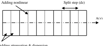
[image:2.595.310.529.600.698.2]Simulation is a computer model of a part of a real-world system [17, 18]. In this paper the simulation is a computer model of a single mode optical fiber link system, includes attenuation function, dispersion function, nonlinear effective function, and propagation function. The method of propagation is divided the path length of signal propagation in steps to add the effective of attenuation, dispersion, and nonlinear in every step. This method called Split-Step Fourier (SSF) [19], as shown in Fig. 1.
Fig. 1: Split-step Fourier method.
The following equations are the attenuation, dispersion, and nonlinear effective equations [20, 21], used in the simulation.
A(z)
Adding attenuation & dispersion
(4) where: α is the attenuation factor.
dz is split-step distance as shown in the figure (1).
( ) (5) For single mode fiber intermodal, or modal, dispersion equal to zero (β1 = 0),
(6)
( ) (
)
( ) (
) (7)
where c is the velocity of light free space. D2 is the second order dispersion.
D3 is the third order dispersion.
(8)
where I = |signal|2
n2 is the nonlinear factor. Aeff is the effective
cross-section area of the fibres' core.
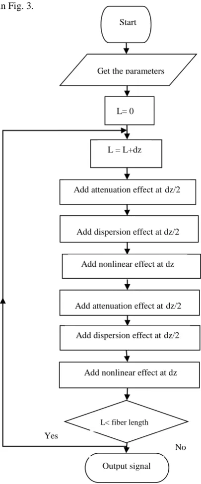
The simulation program of propagation of the light signal in the fiber optic system is given by the flow chart shown in Fig. 2, using Visual C++, [22, 23]. The attenuation effect can be added either in time domain or in frequency domain. In the simulation the attenuation has been added in time domain. But when the dispersion effect is added, it must be add in frequency domain. While the nonlinear effect is add in time domain. The signal transform from domain to another domain can made using Fast Fourier Transform (FFT) [24].
V. THE INPUT SIGNALS
The input signals are the signals that will transmit through the fiber link, or, the output signals of the light sources. These signals are converted in to a shape that the computer can deal with it. So, the input signal must first be represented in the form of a numeric array. The array contains samples of the amplitude profile at N equally spaced points. The sampling resolution must be fine enough to resolve all spatial features of the amplitude profile, at the same time it must sparse enough to allow reasonable processing speed on a computer. The type of pulses that used in the simulation is Gaussian pulse [25]:
( ) { ( ) } (9)
With full width at half amplitude:
√ (10) and with root-mean-square pulse width:
√ (11)
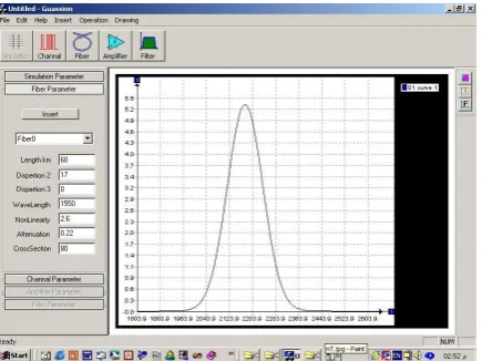
[image:3.595.308.511.198.687.2]The Gaussian pulse is used because the optical sources have a distribution of power with wavelength that is approximately Gaussian distribution in form, as shown in Fig. 3.
Fig. 2: The computer programs flowchart. L= 0
Start
No Yes
Add attenuation effect atdz/2
Add dispersion effect at dz/2
Add nonlinear effect at dz
Add attenuation effect atdz/2
Add dispersion effect atdz/2
Add nonlinear effect at dz
L< fiber length
Output signal Get the parameters
Fig. 3: Gaussian pulse.
VI. SIMULATION RESULTS
[image:4.595.304.527.49.215.2]In the simulation, Gaussian pulse has taken as an input signal and studies all effects that change its shape due to attenuation, dispersion and nonlinearly. In the first example the output taken at a distance 25 km, while in the second example the output is taken at a distance 60 km. Fig.s (4 - 11) illustrate the effects of attenuation, dispersion, and nonlinearity of the fiber for the two examples.
Fig. 4: Attenuation effects at 25 km distance.
[image:4.595.304.527.239.403.2]Fig. 5: Attenuation effects at 60 km distance.
[image:4.595.75.291.349.512.2]Fig. 6: Dispersion effects at 25 km distance.
Fig. 7: Dispersion effects at 60 km distance.
Fig. 8: Nonlinear effects at 25 km distance.
[image:4.595.305.524.426.587.2] [image:4.595.74.292.533.696.2] [image:4.595.306.521.611.769.2]Fig. 10: All effects at 25 km distance.
Fig. 11: All effects at 60 km distance.
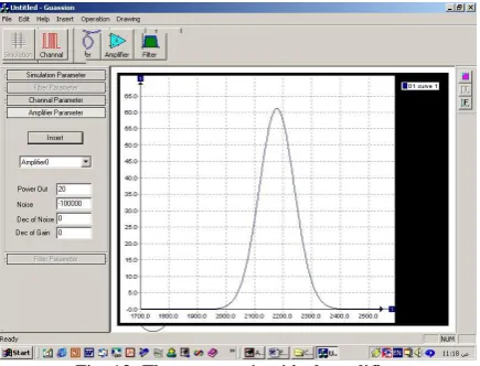
It is clear from the comparison between the results of the two examples that the attenuation, the dispersion and the nonlinearly effects increase when the distance of communication through the fiber optics is increase. Therefore, repeaters are necessary for long-distances fiber optic systems when the signals be very weak. Optical in-line amplifiers must be used as repeaters for compensating the attenuation affects. But the amplifiers add noise, so it is necessary to use filters after the amplification of the signal. The filter removes the effects of the noise, as shown in Fig.s (12-14).
[image:5.595.306.522.234.404.2]Fig. 12: The output using ideal amplifier.
[image:5.595.75.290.236.410.2]Fig. 13: The output using practical amplifier.
Fig. 14: The output using amplifier and filter.
VII. CONCLUSION
In this paper, simulation methods are presented on a single mode optical fiber link system, using VC++. The signal with wavelength of 1550 micrometer was used, to study the effects of attenuation, dispersion, and nonlinear through the fiber optic length by numerical simulations. The results indicate that these effects increase with increasing the distance through the fiber optic length. As propagation continues attenuation increases. Ultimately, the propagating signal is attenuated until it is at some minimal, detectable, level. At this distance we used amplifiers to regenerate the optical signal and to eliminate the effects of the attenuation. We supposed this distance at 25 km in the first example, and 60 km in the second example.
REFERENCES
[1] R.F. Kearns and E.E. Basch, "Computer Analysis of Single-Mode Fiber Optic Systems", GTE Laboratories Incorporated, 40 Sylvan Road, Waltham, MA 02254, 1988, Page(s): 579-583.
[2] G. Keiser, “Optical Fiber Communications”, Singapore: McGraw-Hill, 2nd edition, 1991.
[3] S, Nilsson-Gistoik, “Optical Fiber Theory for Communication Networks", Sweden: Ericsson, 1994. [4] L.Harte, & D.Eckard, "Fiber Optic Basics, Technology,
Systems and Installation", Athos Publishing, USA, 2006.
[image:5.595.73.291.575.741.2][6] S. Yelanin, V. Katok, and O. Ometsinska, "Length Optimization of Fiber Optic Regeneration Section Considering Dynamic Broadening of Optical Transmitter Spectrum", Proceedings of 2004 6th International Conference on Transparent Optical Networks, Volume 2, Issue, 4-8 July 2004, Page(s): 172 - 176 vol.2, 2004.
[7] M.I. Baig,; T.Miyauchi, and M. Imai, " Distributed measurement of chromatic dispersion along an optical fiber transmission system" Proceedings of 2005 IEEE/LEOS Workshop on Fibers and Optical Passive Components, Volume , Issue , 22-24 June 2005 Page(s): 146 – 151, 2005.
[8] Sabah H. S. Albazzaz, "Fundamental of Optical Communication Systems", In Arabic Language, University of Science and Technology, Yaman, 2008. [9] F. Yaman; Q. Lin; S. Radic; and G.P. Agrawal,
"Impact of Dispersion Fluctuations on Dual-Pump Fiber-Optic Parametric Amplifiers", Photonics Technology Letters, IEEE Volume 16, Issue 5, Page(s):1292 – 1294, May 2004.
[10] V.B. Katok,M. Kotenko,and O.Kotenko, "Features of Calculation of Wideband Dispersion Compensator for Fiber-Optic Transmission System", 3rd International Workshop on Laser and Fiber-Optical Networks Modeling, Proceedings of LFNM 2001. Page(s):88 – 91, 2001.
[11] V. Alwayn, "Fiber-Optic Technologies", Cisco Press, 2004.
[12] E. Desurvire, "Erbium-Doped Fiber Amplifiers, Principles and Applications", John Wiely and Sons, 2008.
[13] N. K. Dutta, and Q. Wang, "Semiconductor Optical Amplifiers", University of Connecticut Press, USA, 2006.
[14] Y. J. He and H. Z. Wang, "Solution Phase Jitter Control Use of Super-Gaussian Filters", State Key Laboratory of Optoelectronic Materials and Technologies, Zhongshan (Sun Yat-Sen) University, Guangzhou 510275, China, 2005.
[15] C. Qiaoqiao, J. Xiaofeng, C. Hao, and Z Xianmin, "Tunable Fiber Fabry-Perot Filter for Optical Carrier-Suppression and Single-Sideband Modulation in Radio over Fiber Links", International Journal of Infrared and Millimeter Waves, Volume 27, Number 3, pp. 381-390 (10), March 2006.
[16] B. A. Usievich, V. A. Sychugov, O. Parriaux, J. K. Nurligareev, "A Narrow-Band Optical Filter Based on Fabry-Perot Interferometer with One Waveguide-Grating Mirror", Quantum Electron, Volume 33, Number 8, pp. 695-698, 2003.
[17]S. M. Rossi, E. Moschim, "Simulation of High Speed Optical Filter Systems Using PC-SIMFO", Proceedings of 47th Electronic Components and Technology Conference, pp. 1289-1294, 18-21 May 1997.
[18] H. Zheng, "Simulation of Optical Fiber Transmission Systems Using SPW on an HP Workstation", Simulation, Volume 71m Number 5, pp. 312-315, 1998.
[19] R. Min, "A Modified Split-Step Fourier Method for Optical Pulse Propagation with Polarization Mode Dispersion", Chinese Physics, Number 12, pp. 502-506, 2003.
[20] Document No. 4929264/2004 United States, "Apparatus for Reducing Optical-Fiber Attenuation", USA, 2004.
[21] G.P. Agrawal, “Nonlinear Fiber Optics”, 3rd editions, San Digo: CA, Academic Press, USA, 2001).
[22] D. J. Kruglinski, S. Wingo, and G. Shepherd, “Programming Microsoft Visual C++”, (Washington, Microsoft Press, 5th edition, 1998).
[23] D. J. Kruglinski, “Development Program Visual C++”, (Washington, Microsoft Press, 1999).