Abstract—In this paper a human locomotion system
cinematic analysis is presented, in order to obtain the cinematic joints motion laws. This cinematic analysis is performed for a 4 years old child in the walking activity case. The obtained results are used for a new knee modular orthosis prototype validation.
Index Terms—cinematic, modular orthosis, human
locomotion system, biomechanics
I. INTRODUCTION
IFFERENT human locomotion system cinematic analyses have been developed through diverse methods [1], [2], [3], [5], [12] and [14].
In this paper a human locomotion system cinematic analysis is performed in the walking case of a 4 years old child. The research aim is to design a new knee orthosis which will be used by children that needs a temporal recovery through therapeutic procedures only for walking activity. The children are permanently in growth and that is the main fact that restricts the orthosis design research area. For this we propose here the development of a new orthosis type which consists in modules that can be modified by depending the chidrens age, sex, weight, height, etc. For this is necessary to study the whole locomotion system from a cinematic viewpoint when perform a single gait.
A cinematic analysis of a mechanical model consists in solving two important problems: cinematic direct problem and cinematic inverse problem. The cinematic direct problem’s frame, the displacements from cinematic joint are known, and it will be determined the positions – orientation, speeds and accelerations of the mechanism elements or some characteristic points onto the analyzed mechanism.
The cinematic inverse problem, cinematic parameters for some characteristic points motion are known, and it will be determined the cinematic joints relative motions parameters. With these, in the cinematic analysis context, we identify many problems such as: positional problem, speed problem, accelerations problem. Each of these problems presents a direct or inverse aspect.
Manuscript received April 2, 2012. This work was supported by the strategic grant POSDRU/89/1.5/S/61968, Project ID61968 (2009), co-financed by the European Social Fund within the Sectorial Operational Program Human Resources Development 2007-2013.
C. Copilusi is with the Faculty of Mechanics, University of Craiova. Calea Bucuresti street no. 113. Romania (corresponding author to provide phone: +04 0747222771; e-mail: cristache03@yahoo.co.uk).
II. HUMAN LOCOMOTION SYSTEM CINEMATIC ANALYSIS
The method used here has a flexible character and assures an interface for dynamic analysis especially for finite element modeling of spatial and planar mobile mechanical systems [6], [7], [8] and [9].
For the cinematic analysis the cinematic model presented in figure 1, will be considered. The cinematic analysis will be performed for walking; only one gait when a foot is fixed with the ground and the other perform the desired motion. The cinematic parameters variation laws were obtained by processing with the MAPLE software aid the mathematical models which are defining the human locomotion system experimentally cinematic analysis.
[image:1.595.313.538.386.756.2]From a structural viewpoint, the cinematic chain it consists in 16 rotation joints.
Fig. 1. Human locomotion system cinematic model.
Design of a New Knee Modular Orthotic Device
from Cinematic Considerations
C. Copilusi
The connectivity order will be: OT – 1 – 2 – 3 – 4 – 5 – 6 – 7 – 8– 9 – 10 – 11 – 12 – 13 – 14 – 15 – 16.
A. Position calculus
The position vectors are:
S ,S ,S
S
W
. S ; W r r , r , r r ; W r r , r , r r ; W r r , r , r r ; W r r , r , r r ; W r r , r , r r ; W r r , r , r r ; W r r , r , r r ; W r r , r , r r ; W r r , r , r r ; W r r , r , r r ; W r r , r , r r ; W r r , r , r r ; W r r , r , r r ; W r r , r , r r ; W r r , r , r r ; W r r , r , r r 16 T 17 z 17 y 17 x 17 17 15 T 16 z 16 y 16 x 16 16 14 T 15 z 15 y 15 x 15 15 13 T 14 z 14 y 14 x 14 14 12 T 13 z 13 y 13 x 13 13 11 T 12 z 12 y 12 x 12 12 10 T 11 z 11 y 11 x 11 11 9 T 10 z 10 y 10 x 10 10 8 T 9 z 9 y 9 x 9 9 7 T 8 z 8 y 8 x 8 8 8 T 7 z 7 y 7 x 7 7 5 T 6 z 6 y 6 x 6 6 4 T 5 z 5 y 5 x 5 5 3 T 4 z 4 y 4 x 4 4 2 T 3 z 3 y 3 x 3 3 1 T 2 z 2 y 2 x 2 2 OT T 1 z 1 y 1 x 1 1 (1)The OT R
r vector, has the following expression:
17 16 15 14 13 12 11 10 9 8 7 6 5 4 3 2 1 OT R S r r r r r r r r r r r r r r r r r (2)
Changing the versors base at crossing from a reference coordinate system to another (introducing the coordinate transformation matrices):
W1
AOT1
WOT; (3)
W2
A12
W1
AOT2
WOT; (4)
W3
A23
W2
AOT3
WOT; (5)
W4
A34
W3
AOT4
WOT; (6)
W5
A45
W4
AOT5
WOT; (7)
W6
A56
W5
AOT6
WOT; (8)
W7
A67
W6
AOT7
WOT; (9)
W8
A78
W7
AOT8
WOT; (10)
W9
A89
W8
AOT9
WOT; (11)
W10
A910
W9
AOT10
WOT; (12)
W11
A1011
W10
AOT11
WOT; (13)
W12
A1112
W11
AOT12
WOT; (14)
W13
A1213
W12
AOT13
WOT; (15)
W14
A1314
W13
AOT14
WOT; (16)
W15
A1415
W14
AOT15
WOT; (17)
W16
A1516
W15
AOT16
WOT; (18)
W17
A1617
W16
AOT17
WOT. (19)By analyzing (3) to (19) we observe that:
A
A
A
; A
A
A
. ; A A A ; A A A ; A A A ; A A A ; A A A ; A A A ; A A A ; A A A ; A A A ; A A A ; A A A ; A A A ; A A A ; A A A 15 OT 1617 16 OT 14 OT 1516 15 OT 13 OT 1415 14 OT 13 OT 1314 14 OT 12 OT 1213 13 OT 11 OT 1112 12 OT 10 OT 1011 11 OT 9 OT 910 10 OT 8 OT 89 9 OT 7 OT 78 8 OT 6 OT 67 7 OT 5 OT 56 6 OT 4 OT 45 5 OT 3 OT 34 4 OT 1 OT 23 3 OT OT 12 2 OT (20)Based on (20) we identify the coordinates transformation matrices for each cinematic joints, with i,i190, and
. 16 , 1
i Point: A, B, C, D, E, F, G, H, I, J, K, L, M, N, O, P
and R positions in rapport with TOT coordinate system, bounded to the left foot, will be identified through the (21) to (28). Similarly, we obtain the displacements of other joint centre points. The displacement for R point is given by (29).
r
W ; rAOT 1T OT
(21)
r
W
r
A
W ;r OT1 OT
T 2 OT T 1 O B
T
(22)
r
A A
W ;W A r W r r OT 1 OT 12 T 3 OT 1 OT T 2 OT T 1 OT C (23)
r A A
W r A A A
W ; W A r W r r OT 1 OT 12 23 T 4 OT 1 OT 12 T 3 OT 1 OT T 2 OT T 1 OT D (24)
r A A A A
W ;W A A A r W A A r W A r W r r OT 1 OT 12 23 34 T 5 OT 1 OT 12 23 T 4 OT 1 OT 12 T 3 OT 1 OT T 2 OT T 1 OT E (25)
W
r
A A A A A
W ; A A A A r W A A A r W A A r W A r W r r OT 1 OT 12 23 34 45 T 6 OT 1 OT 12 23 34 T 5 OT 1 OT 12 23 T 4 OT 1 OT 12 T 3 OT 1 OT T 2 OT T 1 OT F (26)
r
A A A A A A
W ; W A A A A A r W A A A A r W A A A r W A A r W A r W r r OT 1 OT 12 23 34 45 56 T 7 OT 1 OT 12 23 34 45 T 6 OT 1 OT 12 23 34 T 5 OT 1 OT 12 23 T 4 OT 1 OT 12 T 3 OT 1 OT T 2 OT T 1 OT G (27)
A A A
W ;
A A A A A A A
W
.A A A A A A A A A S W A A A A A A A A A A A A A A A r W A A A A A A A A A A A A A A r W A A A A A A A A A A A A A r W A A A A A A A A A A A A r W A A A A A A A A A A A r W A A A A A A A A A A r W A A A A A A A A A r W A A A A A A A A r W A A A A A A A r W A A A A A A r W A A A A A r W A A A A r W A A A r W A A r W A r W r r OT 1 OT 12 23 34 45 56 67 78 89 910 1011 1112 1213 1314 1415 1516 T 17 OT 1 OT 12 23 34 45 56 67 78 89 910 1011 1112 1213 1314 1415 T 16 OT 1 OT 12 23 34 45 56 67 78 89 910 1011 1112 1213 1314 T 15 OT 1 OT 12 23 34 45 56 67 78 89 910 1011 1112 1213 T 14 OT 1 OT 12 23 34 45 56 67 78 89 910 1011 1112 T 13 OT 1 OT 12 23 34 45 56 67 78 89 910 1011 T 12 OT 1 OT 12 23 34 45 56 67 78 89 910 T 11 OT 1 OT 12 23 34 45 56 67 78 89 T 10 OT 1 OT 12 23 34 45 56 67 78 T 9 OT 1 OT 12 23 34 45 56 67 T 8 OT 1 OT 12 23 34 45 56 T 7 OT 1 OT 12 23 34 45 T 6 OT 1 OT 12 23 34 T 5 OT 1 OT 12 23 T 4 OT 1 OT 12 T 3 OT 1 OT T 2 OT T 1 OT R (29)
B. Speed calculus
We follow to determine the R point speed depending with OT
T reference system. For this we differentiate successively (21) to (29), but for achieve this calculus is necessary to build the anti symmetric matrices for each joint, like the form from (30).
0 0 0 Cxj Cxj Cxi Cxi Cxi Cxi Cxi ~
, withi,j1,16. (30)
For this:
A
.A ; A A ; A A ; A A ; A A ; A A ; A A ; A A ; A A ; A A ; A A ; A A ; A A ; A A ; A A ; A A ; A A 17 OT ~ 1617 17 OT 16 OT ~ 1516 16 OT 15 OT ~ 1415 15 OT 13 OT ~ 1314 14 OT 13 OT ~ 1213 13 OT 12 OT ~ 1112 12 OT 11 OT ~ 1011 11 OT 10 OT ~ 910 10 OT 9 OT ~ 89 9 OT 8 OT ~ 78 8 OT 7 OT ~ 67 7 OT 6 OT ~ 56 6 OT 5 OT ~ 45 5 OT 4 OT ~ 34 4 OT 3 OT ~ 23 3 OT 2 OT ~ 12 2 OT 1 OT ~ 1 OT 1 OT (31)
By differentiating (21) to (29) for each joint centre point we obtain the speed equations. For A, B and C, we will obtain the speed (32), (33) and (34). Similarly, we obtain the velocities of other joint centre points. The velocity for R
point is given by (35).
; 0 vAOT
(32)
r
A
W ; 0v OT1 OT
~ 1 OT T 2 OT
B
(33)
A
W ;r W A r 0 v OT 2 OT ~ 12 T 3 OT 1 OT ~ 1 OT T 2 OT C (34)
A
W .S W A r W A r W A r W A r W A r W A r W A r W A r W A r W A r W A r W A r W A r W A r W A r 0 v OT 16 OT ~ 1516 T 17 OT 15 OT ~ 1415 T 16 OT 14 OT ~ 1314 T 15 OT 13 OT ~ 1213 T 14 OT 12 OT ~ 1112 T 13 OT 11 OT ~ 1011 T 12 OT 10 OT ~ 910 T 11 OT 9 OT ~ 89 T 10 OT 8 OT ~ 78 T 9 OT 7 OT ~ 67 T 8 OT 6 OT ~ 56 T 7 OT 5 OT ~ 45 T 6 OT 4 OT ~ 34 T 5 OT 3 OT ~ 23 T 4 OT 2 OT ~ 12 T 3 OT 1 OT ~ 1 OT T 2 OT R (35)
C. Acceleration calculus
These will be obtained by differentiating successively the speed equations. For A, and B, we will obtain the accelerations (36) and (37). Similarly, we obtain the accelerations of other joint centre points. The acceleration for R point is given by (38).
; 0 aAOT
(36)
A
W .
W
.A S
W A S
W A r
W A
r W A r
W A
r W A r
W
A r
W A r
W A r
W A
r W A r
W A
r W A r
W A
r W A r
W A
r W A r
W A
r W A r
W A
r W A r
W A
r W A r
W A
r W A r
W A
r W A r
W A
r W A r
W A
r W A r
0 a
OT
16 OT ~ 1516 ~ 1516 T 17 OT 16 OT ~ 1516 T 17
OT 15 OT ~ 1415 ~ 1415 T 16 OT 15 OT ~ 1415
T 16 OT 14 OT ~ 1314 ~ 1314 T 15 OT 14 OT
~ 1314 T 15 OT 13 OT ~ 1213 ~ 1213 T 14 OT
13 OT ~ 1213 T 14 OT 12 OT ~ 1112 ~ 1112 T 13
OT 12 OT ~ 1112 T 13 OT 11 OT ~ 1011 ~ 1011
T 12 OT 11 OT ~ 1011 T 12 OT 10 OT ~ 910
~ 910 T 11 OT 10 OT ~ 910 T 11 OT 9 OT
~ 89 ~ 89 T 10 OT 9 OT ~ 89 T 10 OT 8 OT
~ 78 ~
78 T 9 OT 8 OT ~ 78 T 9 OT 7 OT
~ 67 ~
67 T 8 OT 7 OT ~
67 T 8 OT 6 OT
~ 56 ~ 56 T 7 OT 6 OT ~
56 T 7 OT 5 OT
~ 45 ~ 45 T 6 OT 5 OT ~
45 T 6 OT 4 OT
~ 34 ~ 34 T 5 OT 4 OT ~ 34 T 5 OT 3 OT
~ 23 ~ 23 T 4 OT 3 OT ~
23 T 4 OT 2 OT
~ 12 ~
12 T 3 OT 2 OT ~
12 T 3 OT 1 OT
~ 1 OT ~
1 OT T 2 OT 1 OT ~
1 OT T 2 OT R
(38) III. NUMERICAL PROCESSING
For cinematic analysis, the geometrical elements are known. The computing algorithm was elaborated with the MAPLE aid. The geometrical elements dimensions are in millimeters: LOT=70; L1=65; L2=65; L3=200; L4=5; L5=225;
L6=5; L7=5; L8=220; L9=5; L10=5; L11=225; L12=5; L13=200;
L14=65; L15=65; L16=70. The generalized coordinate system
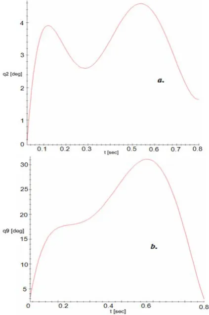
[image:4.595.315.541.49.390.2]variations for the equivalent locomotion system active joints in walking activity’s case are presented in Fig. 3, 4 and 5. These were processed in a 4 years old child. The angular amplitudes of these motion laws were validated by consulting specialty literature data [10].
Fig. 2. Generalized coordinate motion law equivalent with the hip joint for walking activity in the case of a 4 year old child: a-left lower limb; b-right
lower limb.
Fig. 3. Generalized coordinate motion law equivalent with the knee joint for walking activity in the case of a 4 year old child: a-left lower limb;
[image:4.595.320.532.437.756.2]Fig. 4. Generalized coordinate motion law equivalent with the ankle joint for walking activity in the case of a 4 year old child: a-left lower limb;
b-right lower limb.
IV. MODULAR KNEE ORTHOSIS DESIGN
The main requirements for a child orthosis are: to have a simple construction and a reduced weight, easy to achieve the angular amplitude for knee flexion in the walking activity, easy to adjust the dimensions, especially when it is used for children, easy to wear. This knee orthosis model will be used for children locomotion recovery through kinetotherapeutic procedures after some bone fractures or surgical interventions at the lower limb’s level. Also this will be a passive one. For these, an orthosis modular structure was designed in order to add or remove modules for increase or decrease in size. The material which will be used for components is aluminum alloys. For this modular orthosis’ command and control a step by step actuator will be used, and an Arduino microcontroller board. These two elements will form the command and control unit and will be placed in a special box with a backpack. The module design was achieved by taking into account the knee modular orthosis cinematic scheme from figure 5. The orthosis cinematic model has a single mobility degree. The virtual model with all the geometric parts was created in SolidWorks and is shown in figures 5 and 6. A link between the command-control unit and the modular orthosis will be made through flexible cables, one for pull up – cable no: 1 and the other for roll back – cable no: 2. For a 4 years old child, the intermediate module was eliminated from his structure in order to decrease his size. For this, as a geometric model remains only primary and final module, and it will be simulated in MSC ADAMS. An interface between SolidWorks and MSC ADAMS/Autoflex was created, for this model. For simulations, the right limb
[image:5.595.306.543.122.337.2]motion law from Fig. 3-b was applied on the Cable no.1. The femur component of primary module was fixed and a load force equal with 450 Newton was applied on final module (this force was determined in a previous work of the authors according with literature data [9], [10]).
Fig. 5. Knee modular orthosis cinematic scheme and virtual model with components identification.
Fig. 6. The modular orthosis virtual model – lateral view for pulley visualization.
Fig. 7. Cables Von Misses stress, final module angular variation and modular orthosis prototype.
[image:5.595.315.539.367.473.2] [image:5.595.309.547.513.750.2]The maximum Von Misses stress value was 18.0635MPa, which is not so high, and the final module angular motion value was 68.7 degrees (Fig. 7). Also for this virtual model, the final module angular displacement has 46.754 degrees.
V. EXPERIMENTAL TESTS
In order to validate the modular orthosis prototype, a 4 years old child with locomotion disability will perform flexion/extension exercises and the motion laws will be achieved with CONTEMPLAS High Speed Motion Analysis equipment (Machine Elements laboratory - Faculty of Mechanics, University of Craiova). This child has a trauma at the right shank’s level, and also the knee joint was affected. The modular orthosis prototype is presented in Fig. 8. As a template from a database developed in this way, for a healthy 4 years old child the knee angular amplitude on a single gait is represented in Fig. 9. The knee angular amplitude developed by a healthy child for walking was 55 degrees, and in the knee modular orthosis case was 48 degrees.
[image:6.595.92.258.305.417.2]
Fig. 8. Knee modular orthosis prototype images from experimental tests.
Fig. 9. Knee angular amplitude analyzed with CONTEMPLAS Motion Equipment in a 4 year old healthy and invalid child case for a single
gait.
VI. CONCLUSIONS
Through this research, a new orthosis type was validated. The novel elements in this research are: a modern cinematic method for computing joints motion laws; developing an interface in order to transfer the virtual model from SolidWorks software, to MSC ADAMS; using modern equipments for evaluating the human subjects. The CONTEMPLAS Equipment can evaluate from cinematic viewpoint parameters in 3D or 2D environments. This modular orthosis can be modified by adding or removing modules depending on child leg’s size.
The result of this research helps the specialist from neuromotor rehabilitation field, to develop a rehabilitation program for 4 years children lower limbs. So in according with this system gait and posture rehabilitation include
specific muscle training, balance training and coordination. Gait and posture rehabilitation can be assess by CONTEMPLAS system and after can be create individual model for modular orthoses that make more easy the lower limb rehabilitation especially at children because in the same time specific rehabilitation technique include the muscle groups that are involved in devices function. We conclude that existence of mathematic model based on cinematic analysis helps increase the results of gait and posture rehabilitation by helping the locomotion system function.
ACKNOWLEDGMENT
This work was supported by the strategic grant POSDRU/89/1.5/S/61968, Project ID61968 (2009), co-financed by the European Social Fund within the Sectorial Operational Program Human Resources Development 2007-2013.
REFERENCES
[1] R. M., Kiss, L., Kocsis, and Z., Knoll, “Joint kinematics and spatial temporal parameters of gait measured by an ultrasound-based system”. Med. Eng. Phys. Journal, vol. 26. pp. 611–620. 2004. [2] A., Heyn, R. E., Mayagoitia, A. V., Nene, and P. H., Veltink, “The
kinematics of the swing phase obtained from accelerometer and gyroscope measurements”. Proceedings of the 18th Int. Conf. IEEE Engineering in Medicine and Biology Society. pp. 463-464. 1996. [3] G. A., Sohl, and J. E. Bobrow, “A Recursive Multibody Dynamics
and Sensitivity Algorithm for Branched Kinematic Chains”. ASME J. Dyn. Syst., Meas., Control. Vol.123_3. pp. 391–399. 2001.
[4] F. C., Anderson, and M. G., Pandy, “Dynamic Optimization of Human Walking”. J. Biomech. Eng., vol. 123_5. pp. 381–390. 2001. [5] D., Hooman, M., Brigitte, ed. al., “Estimation and Visualization of
Sagittal Kinematics of Lower Limbs Orientation Using Body-Fixed Sensors”. IEEE Transactions On Biomedical Engineering, Vol. 53, No. 7. 2006. pp. 1385–1393.
[6] N., Dumitru, G., Nanu, ed. al., “Mechanisms and mechanical transmissions. Modern and classical design techniques”. Didactic printing house. Bucharest. Romania. Chap. 1. pp. 7-48. 2008. [7] N., Dumitru, A., Margine., “Modeling bases in mechanical
engineering”. Universitaria printing house. Craiova. Romania. pp. 45-108. 2000.
[8] N., Dumitru, M., Cherciu, Z., Althalabi, “Theoretical and Experimental Modelling of the Dynamic Response of the Mechanisms with Deformable Kinematics Elements”. Proceedings of IFToMM, Besancon, France. Paper A-954. 2007.
[9] C., Copilusi, “Researches regarding some mechanical systems applicable in medicine”. PhD. Thesis, Faculty of Mechanics, University of Craiova. Romania. 2009.
[10] M., Williams, “Biomechanics of human motion”. W.B. Saunders Co. Philadelphia and London. U.K. 1996.
[11] C-Y. E., Wang, J. E., Bobrow, D. J., Reinkensmeyer, “Dynamic Motion Planning for the Design of Robotic Gait Rehabilitation”
Journal of Biomechanical Engineering. Vol. 127. 2005.
[12] C-Y. E., Wang J. E., Bobrow, and D. J., Reinkensmeyer, “Swinging from the Hip: Use of Dynamic Motion Optimization in the Design of Robotic Gait Rehabilitation”. IEEE International Conference on Robotics and Automation, vol. 2. 2001. pp. 1433–1438.
[13] C., Copilusi, N., Dumitru, L., Rusu, M., Marin, “Implementation of a cam mechanism in a new human ankle prosthesis structure”.
Proceedings of DAAAM International Conference Vien, Austria. pp 481-483. 2009.
[image:6.595.50.285.439.563.2]