Vipul Ranatunga
Abstract - Finite element analysis of the delamination crack propagation in laminated composites is presented. Fracture mechanics based Virtual Crack Closure Technique (VCCT), and the cohesive element technique, have been used to simulate the delamination initiation and propagation under Mode-I type loading. Detailed description of the parameter selection process for these two techniques with ABAQUS®/Standard is discussed with respect to Mode-I delamination using a double cantilever beam model. Mesh refinement and sensitivity of the mesh size on reaching accurate predictions are highlighted through simulations. The significance of each parameter on the accuracy of the model considering the prediction of crack extension, load versus crack-opening displacement, and the effect of these parameters on reaching a converged and stable solution are discussed.
Index Terms - fracture, delamination, composite damage, cohesive elements, interface damage
I. INTRODUCTION
OMPOSITE materials have been used in aerospace applications to reduce the weight as well as improve the functionality of the structure by tailoring the strength properties. Delamination between plies in laminated composite structures has proven to be one of the major challenges in utilizing composite materials in various applications. Design strategies and effective utilization of laminated composite materials for composite structures rely on the capabilities of predicting the interlaminar failure under various loading and environmental conditions. Mainly in the context of finite element analyses, the goal has been to capture not only the onset (initiation) of delamination, but also the progression. The procedures for numerical modeling of delamination can be divided into two main groups: (1) the models based on direct application of fracture mechanics, and (2) the models within the framework of damage mechanics. One of the most widely used fracture mechanics based approaches is the Virtual Crack Closure Technique [1, 2] (VCCT). This approach is based on Linear Elastic Fracture Mechanics (LEFM) and requires an initial crack to predict the delamination. Another widely used approach for modeling delamination based on damage mechanics is the cohesive elements based on the cohesive zone models [3, 4]. A cohesive damage zone is assumed at the crack tip, and the model relates tractions to displacement jumps at an interface where a crack may take place. Both of these state-of-the-art methods have been incorporated into the ABAQUS® finite element software [5] for the simulation of initiation and extension of delamination.
Manuscript received March 24, 2011; revised April 13, 2011. This work was supported in part by Miami University Center for Advancement of Computational Research. Additionally, software and hardware support was provided by Research Computing Support Group at Miami University.
Author is affiliated with the Department of Engineering Technology, Miami University, Middletown, OH 45042 USA. (Phone: +1 513 727 3448; Fax: +1 513 727 3367; E-mail: [email protected]).
This paper presents the details of modeling composite delamination with both VCCT and cohesive element approaches. Detailed description of parameter selection related to each approach, significance of these parameters, and the details of the experimental work with unidirectional AS4/3501-6 carbon/epoxy system to validate the finite element models are presented in the subsequent sections.
II. VIRTUAL CRACK CLOSURE TECHNIQUE (VCCT) The Virtual Crack Closure Technique uses the principle of Linear Elastic Fracture Mechanics (LEFM) to predict the crack propagation taking place along a predefined surface. VCCT assumes that the strain energy released during a crack extension is the same energy required to close the crack. The fracture initiates at any given node under mixed-mode condition when the equivalent strain energy release rate Geq calculated at any given node exceeds critical
equivalent strain energy rate GCeq calculated based on a
specific mode-mix criterion defined by the user. One such criterion is the Benzeggagh-Kenane [6] law (B-K law) given by
(1)
where GIC and GIIC are the critical energy release rates
associated with pure Mode I and Mode II fracture, respectively. Power Law and Reeder Law are the two other formulae available in ABAQUS® to calculate equivalent strain energy release rate, but only the B-K formula is used in this study.
III. COHESIVE ELEMENT METHOD
Cohesive elements in ABAQUS® are used to model bonded interfaces when the interface thinkness is negligibly small. A traction-separation based constitutive response is defined by an adhesive material with number of material parameters including interfacial penalty stiffness, interfacial strength, and the critical fracture energy. Fig. 1 shows a commonly used traction-separation law where
σ
max is thedebonding strength of the material, and Gc is the the area
under the curve representing fracture energy of the material. Additionally, cohesive model introduces an artificial elastic modulus En, producing elastic deformation prior to the
initiation of damage, which has to be avoided by introducing a relatively high dummy stiffness for interface elements, which is not a material-related parameter. Debond strength and fracture energy for a given material can be determined by experiments. As an example, using a DCB test, debonding value and fracture energy corresponding to Mode-I type crack propagation can be determined. Selecting an arbitrarily soft value for En may introduce a considerable
compliance to the interface, while a higher stiffness may cause spurious traction oscillations [7].
Finite Element Modeling of Delamination Crack
Propagation in Laminated Composites
Fig. 1. Traction-Separation Law used to Define Cohesive Model and the related Parameter
Damage initiation takes place as the degradation of the stiffness begins when the stresses and/or strains satisfy a specified damage initiation criteria. Under the mixed-mode loading, quadratic nominal stress criterion defined by Eq. (2) is used to initiate the damage. When the ratio between nominal stress reaches a value of one, the damage initiates and the criteria is expressed as
(2)
where, indicates that a pure compressive stress state will not initiate damege. Damage evolution represents the rate of stiffness degradation after a damage initiation criteria is reached. Damage evolution is defined by the fracture energy, which is the area under traction-separation curve of the cohesive model. Components of fracture energies associated with each mode of fracture (pure Mode I/Mode II/Mode III) must be specified as a material property similar to VCCT criteria. As an example, the B-K formulation given by Eq (2) can be used for damage evolution. Damage evolution in the cohesive model is captured by a scalar damage variable D. After the damage initiation, the damage variable D monotonically evolves from 0 to 1, and the cohesive elements with a damage variable that has reached this maximum are removed. This element removal process is more appropriate for modeling fracture and separation of components similar to a DCB test. If the elimination process is not needed, cohesive elements can be left in the model after completely damaged, which may be appropriate in cases where it is necessary to resist the interpenetration of the surrounding components. Element removal has been enabled during the current DCB simulations to indicate the crack propagation and the location of the crack tip.
IV. FINITE ELEMENT MODEL
To begin the comparison between the VCCT approach and the cohesive element approach, a transversely isotropic double cantilever beam (DCB) specimen geometry is considered. As shown in Fig. 2, the selected beam has a length (L) of 203 mm width (2W) of 3 mm and thickness of 25.4 mm. The beam includes two sub-laminates, each with a thickness of 1.5 mm and an initial crack length (CL) of 30
mm between the two sub-laminates. Material properties of AS4/3501-6 given in Table 1 are used in the plane-strain finite element models, considering unidirectional fibers aligned with the length direction (Y) of the specimen.
Fig. 2. Geometry of the DCB specimen with applied boundary conditions.
The middle surface between the two sub-laminates is identified as the path for delamination. In order to use the VCCT approach, it is necessary to define an existing crack. The initial crack as indicated in Fig.2 is the initial unbounded surface between the sub-laminates. Both the initial crack and the prospective crack path have to be identified as surfaces in the finite element model when using the VCCT approach. The area representing the two sub-laminates is meshed using reduced integration plane strain (CPE4R) elements. Material properties in Table 1 assumes elastic-orthotropic material model with transverse isotropy.
[image:2.595.310.535.58.131.2]In the case of simulations with ABAQUS® cohesive elements, the geometry shown in Fig. 2 remains the same. In order to define the prospective crack path, a layer of zero-thickness cohesive elements (COH2D4) are been employed along the dotted line in Fig. 2. The remainder of the model is meshed using reduced integration plane strain (CPE4R) elements with the standard ABAQUS® elastic orthotropic model with transverse isotropy, representing the same graphite/epoxy material discussed above.
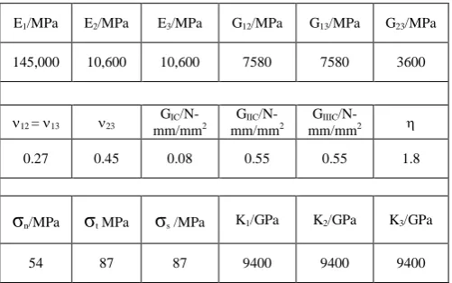
Table 1.
Mechanical properties of AS4/3501-6 and parameters used with traction-separation laws
E1/MPa E2/MPa E3/MPa G12/MPa G13/MPa G23/MPa
145,000 10,600 10,600 7580 7580 3600
ν12 = ν13 ν23
GIC
/N-mm/mm2
GIIC
/N-mm/mm2
GIIIC
/N-mm/mm2 η 0.27 0.45 0.08 0.55 0.55 1.8
σ
n/MPaσ
t MPaσ
s /MPa K1/GPa K2/GPa K3/GPa54 87 87 9400 9400 9400
A. Identification of Control Parameters for VCCT Simulations
It is necessary to identify the optimal values of the control parameters associated with convergence in order to simulate the progressive delamination growth using the VCCT approach. Simulation of crack propagation is a challenging problem and stabilization techniques are required to overcome the convergence difficulties.
Viscous regularization is one such parameter that introduces localized damping to overcome convergence difficulties. Viscosity is added as a factor when specifying the debonding master and slave surfaces, and is often considered as an iterative procedure to set a correct viscosity
σdb
u
G
cσ
δc
δf
[image:2.595.48.255.60.178.2] [image:2.595.305.556.455.612.2]value. Once an appropriate value of viscosity is selected to overcome any convergence issues, it is necessary to compare the energy consumed as the ‘damping energy’ with total strain energy of the model to ensure that the former is not too high in relation to the latter.
Automatic stabilization of an unstable quasi-static problem can also be achieved by the addition of volume-proportional damping factor to the model. An automatic stabilization with a constant damping factor can be included in any nonlinear analysis step in ABAQUS®. The damping factor can be calculated based on the dissipated energy fraction or it can be directly specified as a reasonable estimate. If automatic stabilization is applied to a problem, it is again necessary to ensure that the viscous damping energy is reasonably low compared to the total strain energy of the model. Obtaining an optimal value for the damping factor may require a number of trials until the issues with convergence are solved and the dissipated energy due to stabilization is sufficiently small compared to total strain energy of the model.
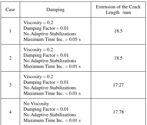
[image:3.595.306.540.53.136.2]An adaptive stabilization scheme is also available in ABAQUS®, where the damping factor is controlled by convergence history and the ratio of energy dissipated by viscous damping to the total strain energy. In order to characterize the effects of these parameters, the following preliminary cases listed in Table 2 have been studied with and without viscous regularization, while maintaining a constant damping factor without adaptive stabilization. In these simulations, a constant displacement of 1.3 mm as shown in Fig. 2 is applied and the length of the crack beyond the initial crack opening (CL in Fig. 2) is observed.
Table 2
Parameters Used for VCCT Simulations with Viscous Regularization and Automatic Stabilization
Case Damping Extension of the Crack Length /mm
1
Viscosity = 0.2 Damping Factor = 0.01 No Adaptive Stabilizations Maximum Time Inc. = 0.05 s
18.5
2
Viscosity = 0.2 Damping Factor = 0.01 No Adaptive Stabilizations Maximum Time Inc. = 0.01 s
18.5
3
Viscosity = 0.2 Damping Factor = 0.01 No Adaptive Stabilizations Maximum Time Inc. = 0.01 s
17.27
4
No Viscosity Damping Factor = 0.01 No Adaptive Stabilizations Maximum Time Inc. = 0.01 s
17.78
The different element sizes and mesh patterns used in these four cases are shown in Fig. 3. The first three cases have used relatively high damping as evident from the comparison of viscous energy to total strain energy as shown in Fig. 4 (only Case 3 is shown), while a much lower energy is consumed as the automatic stabilization energy (static dissipation).
[image:3.595.306.519.165.314.2]a) Case 1 b) Case 2 c) Cases 3 & 4 Fig. 3. Different mesh sizes used in VCCT simulation cases 1-4.
Fig. 4. Comparison of strain energy, viscous energy, and stabilization energy for VCCT Case 3
For these four DCB simulations under displacement control, reaction force verses time is shown in Fig. 5 and the response displays considerable oscillations during delamination propagation.
Fig. 5. Effect of damping, stabilization, and viscosity on reaction force for VCCT cases 1-4
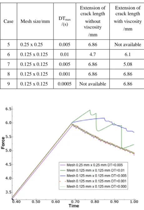
In order to reduce the oscillations observed in the reaction force, a finer mesh has been utilized and another set of simulations have been completed. When an analysis with small mesh is utilized with VCCT, it is necessary to maintain a small time increment. In order to understand the optimal mesh size and maximum allowable time increment, five additional cases have been studied with two different mesh sizes of 0.25 mm x 0.25 mm and 0.125 mm x 0.125 mm with four different maximum allowable time increments as given in the Table 3.
[image:3.595.307.518.398.540.2] [image:3.595.50.292.462.668.2]Table 3
VCCT simulation studies with mesh size, maximum allowable time increment, and the resultant crack length with and without viscosity
Fig. 6. Effect of mesh size and corresponding small time increment required by VCCT cases 5-9
Time increments of 0.001 seconds and 0.0005 seconds produced identical results indicating a maximum time increment of 0.001 seconds is adequate for the selected mesh size of 0.005 inches. Additionally, if a finer mesh is not needed, a time increment of 0.005 could be utilized as proven by 0.25 mm x 0.25 mm mesh size while producing almost identical results according to Fig. 6. The crack extension observed in cases 5, 7, and 8 has been predicted consistently at 6.86 mm while the case 6 with small element size but relatively high time increment produced a much lower crack extension.
[image:4.595.51.282.99.434.2]Also, these crack extension values have been smaller than the values reported under Table 2 with large element size and high viscosity. Therefore, mesh size as well as maximum allowable time increment must be considered in order to obtain smooth and accurate crack propagation with VCCT. VCCT simulation Case 5 reported in Table 3 maintained a viscosity of 0.1 compared to a higher viscosity value of 0.2 used with Case 3 in Table 2. The comparison of viscous dissipation energies with total strain energy for these two cases is shown in Fig. 7. A relatively low ratio of viscous dissipation energy to total strain energy is reported in Case 5, while maintaining a lower oscillation during crack propagation. In contrast, Case 3 displays a higher viscous dissipation and an oscillating response as reported in Fig. 6.
Fig. 7. Comparison of viscous dissipation energy and total strain energy with different viscosity values used in VCCT simulations.
B. Identification of Control Parameters for Cohesive Element Simulations
[image:4.595.324.526.515.602.2]For the cohesive element approach, selection of simulation parameters such as viscous regularization and automatic stabilization must be done by trial and error. Comparison of the stabilization energy and viscous dissipation energy to the overall strain energy of the model for validation of these parameters is also necessary. Furthermore, selection of the interfacial penalty stiffness and interfacial strength values along the normal and shear directions are challenging and discussed in detail by Song et al. [8] for simulations with ABAQUS®. During the present study, a number of finite element simulations have been conducted to identify the necessary minimal damping to avoid convergence issues while accelerating the solution process. Element sizes and viscous damping values used in these simulations are listed in Table 4.
Table 4
Simulations with cohesive elements at different element sizes and damping.
Case Element Size/mm
Viscous Damping
Crack Extension/mm
1 0.25 1e-5 19.56
2 0.25 1e-4 18.29
3 0.25 5e-4 14.73
The variation of energy dissipation due to viscous effects used for automatic stabilization is shown in Fig. 8. According to these comparisons, simulations with a higher viscosity value tends to overpredict the response while producing a smooth load-displacement (time) curve avoiding oscillations, and the solution process is faster. Even though the response reflects small oscillations, a mesh size of 0.25 mm elements is sufficient enough to reach the mesh convergence. According to the values reported on Table 4, the length of the crack extension has been predicted at 19.56 mm by the model with low viscosity. When a significant portion of the energy is consumed as viscous energy, length of the crack has been predicted at a lower value, irrespective of the element size used in these simulations.
Case Mesh size/mm DTmax /(s)
Extension of crack length without viscosity
/mm
Extension of crack length with viscosity
Fig. 8. Dissipation of energy due to static stabilization
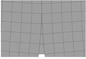
Additionally, the length of the cohesive zone under Mode-I loading can be expressed in terms of material properties as
(3)
where M is a factor that depends on the constitutive laws of the material, and a value of π/4 is used based on Cox and Marshall [9]. E2 is the modulus of elasticity for the material
in transverse direction and
σ
n0 is the nominal strength of the [image:5.595.306.538.57.224.2]material when the deformation is purely normal to the interface. The cohesive zone, as observed with 0.25 mm mesh in Fig. 9, has a length of about 1 mm. According to these simulations with material data reported in Table 1 (and shown in Fig. 9), an element size of 0.25 mm could produce more than four elements along the cohesive zone, representing the fracture process zone accurately.
Fig. 9. Deformed mesh with cohesive zone
V. COMPARISON OF VCCT AND COHESIVE RESULTS
In order to compare the reaction forces predicted by VCCT and cohesive elements, following set of cases has been selected based on the resullts reported in the previous sections. Simulations with VCCT used a mesh size of 0.25 mm, a maximum allowable time increment of 0.005 seconds, and zero viscosity, as verified by simulations reported in Fig. 6. In the case of cohesive elements, same element size of 0.25 mm, a maximum allowable time increment of 0.01 seconds, and a viscosity of 5e-5 have been used for optimal results.
Based on the selected parameters, comparison of reaction forces predicted by the two models are shown in Fig. 10. The local stress distribution observed near the crack-tip for the cohesive model is relatively high compared to VCCT model. Regardless of the disagreement of local stresses near the crack-tip, overall response of these two models remain consistant as evidenced from reaction forces shown in Fig. 10.
Fig. 10. Reaction forces predicted by VCCT and cohesive models
The time taken to complete the execution of each model is shown in Table 5. A significant advantage with execution time is displayed by VCCT model against cohesive model.
Table 5
Total CPU time take for completing a simulation with VCCT and cohesive models
The cohesive model with maximum allowable time of 0.01 seconds took almost five times more CPU time compared to the VCCT simulation with 0.005 second constant time increment. If a large maximum allowable time increment is used with the cohesive models, the solution process becomes unstable due to severe nonlinearities at the verge of a crack initiation. Abaqus/Standard offers a set of stabilization mechanisms to handle nonlinear problems by allowing the user to specify number of solution control parameters such as number of equilibrium iterations (I0) and
number of equilibrium iterations after which the logarithmic rate of convergence check begins (IR). Even with current
increment of 0.01 seconds for the cohesive model, these convergence parameters have to be modified in order to stabilize the solution process.
VI. CONCLUSIONS AND FUTURE WORK
Detailed comparison of VCCT and cohesive element approach for modeling delamination crack propagation is presented in this paper. A simple plane strain DCB delamination simulation was used for the comparison, yet this still required a great deal of operator effort and execution time to obtain reliable results in the case of VCCT and cohesive elements. Based on the results presented in this paper, it is possible to understand the significance of the different parameters needed to fine-tune in order to reach a stable and accurate solution. It has been noticed that the users of these two approaches have experienced considerable difficulty in finding the correct mix of these parameters to achieve a consistently stable solution for delamination crack propagation. Therefore, the detailed procedure provided in this paper will be useful for the beginners to use these approaches effectively. Comparison
Model Total CPU Time/s
VCCT Model 3241
[image:5.595.45.191.434.534.2]of their model predictions against the results presented in this paper will validate the accuracy of their models.
Future work will seek to apply the same two modeling approaches to investigate the delamination crack propagation under Mode-II and mixed-mode loading conditions. Additionally, comparison of these model predictions against experimental results will be completed as a result of the ongoing experiments.
ACKNOWLEDGMENTS
Author would like to acknowledge the support received through Miami University Center for Advancement of Computational Research for sponsoring the research. Also, the software and hardware support received from Research Computing Support Group at Miami University is highly appreciated.
REFERENCES
[1] Rybicki, E. F., Kanninen, M. F., “A finite element calculation of stress intensity factors by a modified crack closure integral”,
Engineering Fracture Mechanics, Vol. 9, 1977, pp. 931-938. [2] Raju, I. S., “Calculation of strain energy release rates with higher
order and singular elements”, Engineering Fracture Mechanics, Vol. 28, 1987, pp. 251-274.
[3] Barenblatt, G. I., “The formation of equilibrium cracks during brittle fracture - general ideas and hypothesis, axially symmetric cracks”,
Prikl. Math. Mekh., Vol. 23, No. 3, 1959, pp. 434-444.
[4] Dugdale, D. S., “Yielding of steel sheets containing slits”, Journal of the Mechanics and Physics of Solids, Vol. 8, 1960, pp. 100-104. [5] Dassault Systemes Simulia Corp., Abaqus Analysis User’s Manual,
Providence, RI, 2011.
[6] Benzeggagh, M. L. and Kenane, M., “Measurement of Mixed-mode Delamination Fracture Toughness of Unidirectional Glass/epoxy Composites with Mixed-mode Bending Apparatus,” Compos. Sci. Technol., Vol. 56, No. 4, pp. 439-449, 1996.
[7] Schellekens, J. J, de Borst, R., “On the numerical integration of interface elements”, International Journal of Numerical Methods in Engineering, Vol. 36, 1992, pp. 43–66.
[8] Song, K., Davila, C. G., and Rose, C. A., “Guidelines and parameter selection for the simulation of progressive delamination”, Abaqus User Conference, Newport, RI, 2008.