Leveraging Cognitive Features for Sentiment Analysis
Abhijit Mishra†, Diptesh Kanojia†,♣, Seema Nagar?, Kuntal Dey?, Pushpak Bhattacharyya†
†Indian Institute of Technology Bombay, India ♣IITB-Monash Research Academy, India
?IBM Research, India
†{abhijitmishra, diptesh, pb}@cse.iitb.ac.in ?{senagar3, kuntadey}@in.ibm.com
Abstract
Sentiments expressed in user-generated short text and sentences are nuanced by subtleties at lexical, syntactic, semantic and pragmatic levels. To address this, we propose to augment traditional features used for sentiment analysis and sarcasm detection, with cognitive features derived from the eye-movement patterns of read-ers. Statistical classification using our en-hanced feature set improves the perfor-mance (F-score) of polarity detection by a maximum of 3.7% and 9.3% on two datasets, over the systems that use only traditional features. We perform feature significance analysis, and experiment on a held-out dataset, showing that cognitive features indeed empower sentiment ana-lyzers to handle complex constructs.
1 Introduction
This paper addresses the task of Sentiment Anal-ysis (SA) - automatic detection of the sentiment polarity as positive versus negative - of user-generated short texts and sentences. Several sen-timent analyzers exist in literature today (Liu and Zhang, 2012). Recent works, such as Kouloumpis et al. (2011), Agarwal et al. (2011) and Barbosa and Feng (2010), attempt to conduct such analy-ses on user-generated content. Sentiment analysis remains a hard problem, due to the challenges it poses at the various levels, as summarized below.
1.1 Lexical Challenges
Sentiment analyzers face the following three chal-lenges at the lexical level: (1)Data Sparsity,i.e., handling the presence of unseen words/phrases. (e.g.,The movie is messy, uncouth, incomprehen-sible, vicious and absurd) (2)Lexical Ambiguity,
e.g.,finding appropriate senses of a word given the context (e.g., His face fell when he was dropped from the team vs The boy fell from the bicycle, where the verb “fell” has to be disambiguated) (3)
Domain Dependency, tackling words that change polarity across domains. (e.g., the word unpre-dictable being positive in case of unpredictable moviein movie domain and negative in case of un-predictable steeringin car domain). Several meth-ods have been proposed to address the different lexical level difficulties by - (a) using WordNet synsets and word cluster information to tackle lex-ical ambiguity and data sparsity (Akkaya et al., 2009; Balamurali et al., 2011; Go et al., 2009; Maas et al., 2011; Popat et al., 2013; Saif et al., 2012) and (b) mining domain dependent words (Sharma and Bhattacharyya, 2013; Wiebe and Mi-halcea, 2006).
1.2 Syntactic Challenges
Difficulty at the syntax level arises when the given text follows a complex phrasal structure and, phrase attachmentsare expected to be resolved be-fore performing SA. For instance, the sentenceA somewhat crudely constructed but gripping, quest-ing look at a person so racked with self-loathquest-ing, he becomes an enemy to his own race. requires processing at the syntactic level, before analyzing the sentiment. Approaches leveraging syntactic properties of text include generating dependency based rules for SA (Poria et al., 2014) and lever-aging local dependency (Li et al., 2010).
1.3 Semantic and Pragmatic Challenges
This corresponds to the difficulties arising in the higher layers of NLP, i.e., semantic and prag-matic layers. Challenges in these layers in-clude handling: (a) Sentiment expressed implic-itly (e.g., Guy gets girl, guy loses girl, audience falls asleep.) (b) Presence of sarcasm and other
forms of irony (e.g., This is the kind of movie you go because the theater has air-conditioning.) and (c) Thwarted expectations (e.g., The acting is fine. Action sequences are top-notch. Still, I consider it as a below average movie due to its poor story-line.).
Such challenges are extremely hard to tackle with traditional NLP tools, as these need both linguistic and pragmatic knowledge. Most at-tempts towards handling thwarting (Ramteke et al., 2013) and sarcasm and irony (Carvalho et al., 2009; Riloff et al., 2013; Liebrecht et al., 2013; Maynard and Greenwood, 2014; Barbieri et al., 2014; Joshi et al., 2015), rely on distant su-pervision based techniques (e.g.,leveraging hash-tags) and/or stylistic/pragmatic features (emoti-cons, laughter expressions such as “lol”etc). Ad-dressing difficulties for linguistically well-formed texts, in absence of explicit cues (like emoticons), proves to be difficult using textual/stylistic fea-tures alone.
1.4 Introducing Cognitive Features
We empower our systems by augmenting cogni-tive features along with traditional linguistic fea-tures used for general sentiment analysis, thwart-ing and sarcasm detection. Cognitive features are derived from the eye-movement patterns of human annotators recorded while they annotate short-text with sentiment labels. Our hypothe-sis is that cognitive processes in the brain are related to eye-movement activities (Parasuraman and Rizzo, 2006). Hence, considering readers’ eye-movement patterns while they read sentiment bearing texts may help tackle linguistic nuances better. We perform statistical classification using various classifiers and different feature combina-tions. With our augmented feature-set, we observe a significant improvement of accuracy across all classifiers for two different datasets. Experiments on a carefully curated held-out dataset indicate a significant improvement in sentiment polarity de-tection over the state of the art, specifically text with complex constructs like irony and sarcasm. Through feature significance analysis, we show that cognitive features indeed empower sentiment analyzers to handle complex constructs like irony and sarcasm. Our approach is the first of its kind to the best of our knowledge. We share various resources and data related to this work at http: //www.cfilt.iitb.ac.in/cognitive-nlp
The rest of the paper is organized as follows. Section 2 presents a summary of past work done in traditional SA and SA from a psycholinguis-tic point of view. Section 3 describes the avail-able datasets we have taken for our analysis. Sec-tion 4 presents our features that comprise both tra-ditional textual features, used for sentiment anal-ysis and cognitive features derived from annota-tors’ eye-movement patterns. In section 5, we dis-cuss the results for various sentiment classification techniques under different combinations of textual and cognitive features, showing the effectiveness of cognitive features. In section 6, we discuss on the feasibility of our approach before concluding the paper in section 7.
2 Related Work
Sentiment classification has been a long standing NLP problem with both supervised (Pang et al., 2002; Benamara et al., 2007; Martineau and Finin, 2009) and unsupervised (Mei et al., 2007; Lin and He, 2009) machine learning based approaches ex-isting for the task.
Supervised approaches are popular because of their superior classification accuracy (Mullen and Collier, 2004; Pang and Lee, 2008) and in such approaches, feature engineering plays an impor-tant role. Apart from the commonly used bag-of-words features based on unigrams, bigrams etc. (Dave et al., 2003; Ng et al., 2006), syntactic prop-erties (Martineau and Finin, 2009; Nakagawa et al., 2010), semantic properties (Balamurali et al., 2011) and effect of negators. Ikeda et al. (2008) are also used as features for the task of sentiment classification. The fact that sentiment expression may be complex to be handled by traditional fea-tures is evident from a study of comparative sen-tences by Ganapathibhotla and Liu (2008). This, however has not been addressed by feature based approaches.
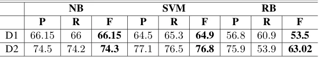
NB SVM RB
P R F P R F P R F
D1 66.15 66 66.15 64.5 65.3 64.9 56.8 60.9 53.5
[image:3.595.136.464.63.123.2]D2 74.5 74.2 74.3 77.1 76.5 76.8 75.9 53.9 63.02
Table 1: Classification results for different SA systems for dataset 1 (D1) and dataset 2 (D2). P→
Precision, R→Recall, F→F˙score
(2013) propose a studied the cognitive aspects if Word Sense Disambiguation (WSD) through eye-tracking. Earlier, Mishra et al. (2013) measure translation annotation difficulty of a given sen-tence based on gaze input of translators used to label training data. Klerke et al. (2016) present a novel multi-task learning approach for sentence compression using labelled data, while, Barrett and Søgaard (2015) discriminate between gram-matical functions using gaze features. The recent advancements in the literature discussed above, motivate us to explore gaze-based cognition for sentiment analysis.
We acknowledge that some of the well perform-ing sentiment analyzers use Deep Learnperform-ing tech-niques (like Convolutional Neural Network based approach by Maas et al. (2011) and Recursive Neural Network based approach by dos Santos and Gatti (2014)). In these, the features are automat-ically learned from the input text. Since our ap-proach is feature based, we do not consider these approaches for our current experimentation. Tak-ing inputs from gaze data and usTak-ing them in a deep learning setting sounds intriguing, though, it is be-yond the scope of this work.
3 Eye-tracking and Sentiment Analysis Datasets
We use two publicly available datasets for our ex-periments. Dataset1has been released by Mishra et al. (2016) which they use for the task ofsarcasm understandability prediction. Dataset2 has been used by Joshi et al. (2014) for the task of sentiment annotation complexity prediction. These datasets contain many instances with higher level nuances like presence of implicit sentiment, sarcasm and thwarting. We describe the datasets below.
3.1 Dataset 1
It contains994text snippets with383positive and
611negative examples. Out of this, 350are sar-castic or have other forms of irony. The snippets are a collection of reviews, normalized-tweets and
quotes. Each snippet is annotated by seven par-ticipants with binary positive/negative polarity la-bels. Their eye-movement patterns are recorded with a high qualitySR-Research Eyelink-1000 eye-tracker(sampling rate500Hz). The annotation ac-curacy varies from70%−90%with a Fleiss kappa inter-rater agreement of0.62.
3.2 Dataset2
This dataset consists of1059snippets comprising movie reviews and normalized tweets. Each snip-pet is annotated by five participants with positive, negative and objective labels. Eye-tracking is done using a low quality Tobii T120eye-tracker (sam-pling rate120Hz). The annotation accuracy varies from75%−85% with a Fleiss kappa inter-rater agreement of0.68. We rule out the objective ones and consider 843 snippets out of which 443 are positive and400are negative.
3.3 Performance of Existing SA Systems Considering Dataset -1and2as Test Data
It is essential to check whether our selected datasets really pose challenges to existing senti-ment analyzers or not. For this, we implesenti-ment two statistical classifiers and a rule based classifier to check the test accuracy of Dataset1 and Dataset
plained by Jia et al. (2009) and intensifiers as ex-plained by Dragut and Fellbaum (2014).
Table 1 presents the accuracy of the three sys-tems. The F-scores are not very high for all the systems (especially for dataset 1 that contains more sarcastic/ironic texts), possibly indicating that the snippets in our dataset pose challenges for existing sentiment analyzers. Hence, the selected datasets are ideal for our current experimentation that involves cognitive features.
4 Enhanced feature set for SA
Our feature-set into four categoriesviz. (1) Sen-timent features (2) Sarcasm, Irony and Thwarting related Features (3) Cognitive features from eye-movement (4) Textual features related to reading difficulty. We describe our feature-set below.
4.1 Sentiment Features
We consider a series of textual features that have been extensively used in sentiment literature (Liu and Zhang, 2012). The features are described be-low. Each feature is represented by a unique ab-breviated form, which are used in the subsequent discussions.
1. Presence of Unigrams (NGRAM˙PCA)i.e. Presence of unigrams appearing in each sen-tence that also appear in the vocabulary ob-tained from the training corpus. To avoid overfitting (since our training data size is less), we reduce the dimension to 500 using Principal Component Analysis.
2. Subjective words (Positive words,
Negative words) i.e. Presence of positive and negative words computed against MPQA lexicon (Wilson et al., 2005), a popular lexi-con used for sentiment analysis.
3. Subjective scores (PosScore, NegScore)i.e. Scores of positive subjectivity and negative subjectivity using SentiWordNet (Esuli and Sebastiani, 2006).
4. Sentiment flip count (FLIP) i.e. Number of times words polarity changes in the text. Word polarity is determined using MPQA lexicon.
5. Part of Speech ratios (VERB, NOUN, ADJ, ADV) i.e. Ratios (proportions) of
verbs, nouns, adjectives and adverbs in the text. This is computed using NLTK1.
6. Count of Named Entities (NE)i.e. Number of named entity mentions in the text. This is computed using NLTK.
7. Discourse connectors (DC)i.e. Number of discourse connectors in the text computed us-ing an in-house list of discourse connectors (likehowever,althoughetc.)
4.2 Sarcasm, Irony and Thwarting related Features
To handle complex texts containing constructs irony, sarcasm and thwarted expectations as ex-plained earlier, we consider the following features. The features are taken from Riloff et al. (2013), Ramteke et al. (2013) and Joshi et al. (2015).
1. Implicit incongruity (IMPLICIT PCA)i.e. Presence of positive phrases followed by negative situational phrase (computed using bootstrapping technique suggested by Riloff et al. (2013)). We consider the top 500 prin-cipal components of these phrases to reduce dimension, in order to avoid overfitting. 2. Punctuation marks (PUNC) i.e. Count of
punctuation marks in the text.
3. Largest pos/neg subsequence (LAR) i.e. Length of the largest series of words with po-larities unchanged. Word polarity is deter-mined using MPQA lexicon.
4. Lexical polarity (LP)i.e. Sentence polarity found by supervised logistic regression using the dataset used by Joshi et al. (2015).
4.3 Cognitive features from eye-movement
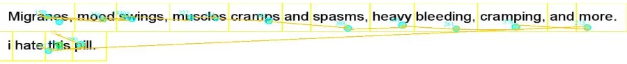
Eye-movement patterns are characterized by two basic attributes: (1)Fixations, corresponding to a longer stay of gaze on a visual object (like char-acters, words etc. in text) (2) Saccades, corre-sponding to the transition of eyes between two fix-ations. Moreover, a saccade is called a Regres-sive Saccadeor simply,Regressionif it represents a phenomenon of going back to a pre-visited seg-ment. A portion of a text is said to be skipped if it does not have any fixation. Figure 1 shows eye-movement behavior during annotation of the given sentence in dataset-1. The circles represent
Figure 1: Snapshot of eye-movement behavior during annotation of an opinionated text. The circles represent fixations and lines connecting the circles represent saccades. Boxes represent Areas of Interest (AoI) which are words of the sentence in our case.
fixation and the line connecting the circles repre-sent saccades. Our cognition driven features are derived from these basic eye-movement attributes. We divide our features in two sets as explained ahead.
4.4 Basic gaze features
Readers’ eye-movement behavior, characterized by fixations, forward saccades, skips and regres-sions, can be directly quantified by simple statis-tical aggregation (i.e., computing features for in-dividual participants and then averaging). Since these behaviors intuitively relate to the cognitive process of the readers (Rayner and Sereno, 1994), we consider simple statistical properties of these factors as features to our model. Some of these features have been reported by Mishra et al. (2016) for modeling sarcasm understandability of read-ers. However, as far as we know, these features are being introduced in NLP tasks like sentiment analysis for the first time.
1. Average First-Fixation Duration per word (FDUR)i.e.Sum offirst-fixation duration di-vided by word count. First fixations are fixa-tions occurring during the first pass reading. Intuitively, an increased first fixation duration is associated to more time spent on the words, which accounts for lexical complexity. This is motivated by Rayner and Duffy (1986).
2. Average Fixation Count (FC)i.e. Sum of fixation counts divided by word count. If the reader reads fast, the first fixation duration may not be high even if the lexical complex-ity is more. But the number of fixations may increase on the text. So, fixation count may help capture lexical complexity in such cases.
3. Average Saccade Length (SL) i.e. Sum of saccade lengths (measured by number of words) divided by word count. Intuitively, lengthy saccades represent the text being structurally/syntactically complex. This is
also supported by von der Malsburg and Va-sishth (2011).
4. Regression Count (REG) i.e. Total num-ber of gaze regressions. Regressions cor-respond to both lexical and syntactic re-analysis (Malsburg et al., 2015). Intuitively, regression count should be useful in captur-ing both syntactic and semantic difficulties. 5. Skip count (SKIP) i.e. Number of words
skipped divided by total word count. Intu-itively, higher skip count should correspond lesser semantic processing requirement (as-suming that skipping is not done intention-ally).
6. Count of regressions from second half to first half of the sentence (RSF)i.e.Number of regressions from second half of the sen-tence to the first half of the sensen-tence (given the sentence is divided into two equal half of words). Constructs like sarcasm, irony of-ten have phrases that are incongruous (e.g. ”The book is so great that it can be used as a paperweight”- the incongruous phrases are ”book is so great” and ”used as a pa-perweight”.. Intuitively, when a reader en-counters such incongruous phrases, the sec-ond phrases often cause a surprisal resulting in a long regression to the first part of the text. Hence, this feature is considered.
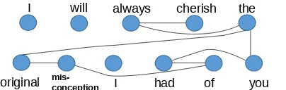
I will always cherish the
[image:6.595.81.283.66.130.2]original mis-conception I had of you
Figure 2: Saliency graph of a human annotator for the sentenceI will always cherish the original mis-conception I had of you.
may help distinguish between sentences with different linguistic subtleties.
4.5 Complex gaze features
We propose a graph structure constructed from the gaze data to derive more complex gaze features. We term the graph asgaze-saliency graphs.
A gaze-saliency graph for a sentence S for a readerR, represented asG = (V, E), is a graph with vertices (V) and edges (E) where each vertex v ∈ V corresponds to a word in S (may not be unique) and there exists an edgee ∈ E between verticesv1 andv2 if R performs at least one sac-cade between the words corresponding tov1and v2. Figure 2 shows an example of such a graph.
1. Edge density of the saliency gaze graph (ED) i.e. Ratio of number of edges in the gaze saliency graph and total number of pos-sible links ((|V|×|V|−1|)/2) in the saliency graph. As,Edge Density of a saliency graph increases with the number of distinct sac-cades, it is supposed to increase if the text is semantically more difficult.
2. Fixation Duration at Left/Source as Edge Weight (F1H, F1S)i.e.Largest weighted gree (F1H) and second largest weighted de-gree (F1S) of the saliency graph considering the fixation duration on the word of nodeiof edgeEij as edge weight.
3. Fixation Duration at Right/Target as Edge Weight (F2H, F2S)i.e.Largest weighted gree (F2H) and second largest weighted de-gree (F2S) of the saliency graph considering the fixation duration of the word of nodeiof edgeEij as edge weight.
4. Forward Saccade Count as Edge Weight (FSH, FSS) i.e. Largest weighted degree (FSH) and second largest weighted degree (FSS) of the saliency graph considering the number of forward saccades between nodesi andjof an edgeEij as edge weight..
5. Forward Saccade Distance as Edge Weight (FSDH, FSDS)i.e. Largest weighted degree (FSDH) and second largest weighted degree (FSDS) of the saliency graph considering the total distance (word count) of forward sac-cades between nodesiandj of an edgeEij
as edge weight.
6. Regressive Saccade Count as Edge Weight (RSH, RSS) i.e. Largest weighted degree (RSH) and second largest weighted degree (RSS) of the saliency graph considering the number of regressive saccades between nodes iandjof an edgeEij as edge weight.
7. Regressive Saccade Distance as Edge Weight (RSDH, RSDS) i.e. Largest weighted degree (RSDH) and second largest weighted degree (RSDS) of the saliency graph considering the number of regressive saccades between nodes iand j of an edge Eij as edge weight.
The ”highest and second highest degree” based gaze features derived from saliency graphs are mo-tivated by our qualitative observations from the gaze data. Intuitively, the highest weighted degree of a graph is expected to be higher if some phrases have complex semantic relationships with others.
4.6 Features Related to Reading Difficulty
Eye-movement during reading text with sentiment related nuances (like sarcasm) can be similar to text with other forms of difficulties. To address the effect of sentence length, word length and syllable count that affect reading behavior, we consider the following features.
1. Readability Ease (RED)i.e. Flesch Read-ability Ease score of the text (Kincaid et al., 1975). Higher the score, easier is the text to comprehend.
2. Sentence Length (LEN) i.e. Number of words in the sentence.
We now explain our experimental setup and re-sults.
5 Experiments and results
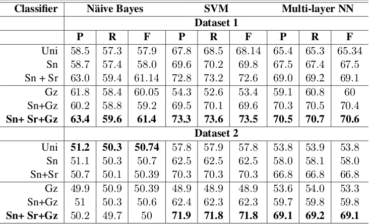
Classifier N¨aive Bayes SVM Multi-layer NN Dataset 1
P R F P R F P R F
Uni 58.5 57.3 57.9 67.8 68.5 68.14 65.4 65.3 65.34
Sn 58.7 57.4 58.0 69.6 70.2 69.8 67.5 67.4 67.5
Sn + Sr 63.0 59.4 61.14 72.8 73.2 72.6 69.0 69.2 69.1
Gz 61.8 58.4 60.05 54.3 52.6 53.4 59.1 60.8 60
Sn+Gz 60.2 58.8 59.2 69.5 70.1 69.6 70.3 70.5 70.4
Sn+ Sr+Gz 63.4 59.6 61.4 73.3 73.6 73.5 70.5 70.7 70.6 Dataset 2
Uni 51.2 50.3 50.74 57.8 57.9 57.8 53.8 53.9 53.8
Sn 51.1 50.3 50.7 62.5 62.5 62.5 58.0 58.1 58.0
Sn+Sr 50.7 50.1 50.39 70.3 70.3 70.3 66.8 66.8 66.8
Gz 49.9 50.9 50.39 48.9 48.9 48.9 53.6 54.0 53.3
Sn+Gz 51 50.3 50.6 62.4 62.3 62.3 59.7 59.8 59.8
[image:7.595.116.482.63.286.2]Sn+ Sr+Gz 50.2 49.7 50 71.9 71.8 71.8 69.1 69.2 69.1
Table 2: Results for different feature combinations. (P,R,F)→Precision, Recall, F-score. Feature labels Uni→Unigram features, Sn→Sentiment features, Sr→Sarcasm features and Gz→Gaze features along with features related to reading difficulty
the Weka (Hall et al., 2009) and LibSVM (Chang and Lin, 2011) APIs. Several classifier hyperpa-rameters are kept to the default values given in Weka. We separately perform a 10-fold cross val-idation on both Dataset 1 and 2 using different sets of feature combinations. The average F-scores for the class-frequency based random classifier are
33% and 46.93% for dataset 1 and dataset 2 re-spectively.
The classification accuracy is reported in Ta-ble 2. We observe the maximum accuracy with the complete feature-set comprising Sentiment, Sar-casm and Thwarting, and Cognitive features de-rived from gaze data. For this combination, SVM outperforms the other classifiers. The novelty of our feature design lies in (a) First augmenting sar-casm and thwarting based features (Sr) with sen-timent features (Sn), which shoots up the accu-racy by3.1%for Dataset1 and7.8%for Dataset2 (b) Augmenting gaze features withSn+Sr, which further increases the accuracy by0.6%and1.5%
for Dataset 1 and 2 respectively, amounting to an overall improvement of 3.7% and 9.3% re-spectively. It may be noted that the addition of gaze features may seem to bring meager improve-ments in the classification accuracy but the im-provements are consistent across datasets and sev-eral classifiers. Still, we speculate that aggregating various eye-tracking parameters to extract the cog-nitive features may have caused loss of
informa-tion, there by limiting the improvements. For ex-ample, the graph based features are computed for each participant and eventually averaged to get the graph features for a sentence, thereby not lever-aging the power of individual eye-movement pat-terns. We intend to address this issue in future.
Since the best (Sn+Sr+Gz) and the second best feature (Sn+Sr) combinations are close in terms of accuracy (difference of0.6%for dataset 1and1.5%for dataset2), we perform a statistical significance test using McNemar test (α = 0.05). The difference in the F-scores turns out to be strongly significant with p = 0.0060 (The odds ratio is 0.489, with a 95% confidence interval). However, the difference in the F-scores is not sta-tistically significant (p = 0.21) for dataset2 for the best and second best feature combinations.
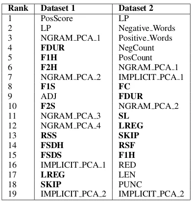
5.1 Importance of cognitive features
We perform a chi-squared testbased feature sig-nificance analysis, shown in Table 3. For dataset 1,
10out of the top20ranked features are gaze-based features and for dataset 2,7out of top20features are gaze-based, as shown in bold letters. More-over, if we consider gaze features alone for fea-ture ranking using chi-squared test, feafea-tures FC, SL,FSDH,FSDS,RSDHandRSDSturn out to be insignificant.
hypoth-Rank Dataset 1 Dataset 2
1 PosScore LP
2 LP Negative Words
3 NGRAM PCA 1 Positive Words
4 FDUR NegCount
5 F1H PosCount
6 F2H NGRAM PCA 1
7 NGRAM PCA 2 IMPLICIT PCA 1
8 F1S FC
9 ADJ FDUR
10 F2S NGRAM PCA 2
11 NGRAM PCA 3 SL
12 NGRAM PCA 4 LREG
13 RSS SKIP
14 FSDH RSF
15 FSDS F1H
16 IMPLICIT PCA 1 RED
17 LREG LEN
18 SKIP PUNC
[image:8.595.83.280.59.264.2] [image:8.595.102.261.341.398.2]19 IMPLICIT PCA 2 IMPLICIT PCA 2 Table 3: Features as per their ranking for both Dataset 1 and Dataset 2. Integer values N in NGRAM PCA N and IMPLICIT PCA N repre-sent theNthprincipal component.
Irony Non-Irony
Sn 58.2 75.5
Sn+Sr 60.1 75.9
Gz+Sn+Sr 64.3 77.6
Table 4: F-scores on held-out dataset for Com-plex Constructs (Irony), Simple Constructs (Non-irony)
esized earlier, we repeat the experiment on a held-out dataset, randomly derived from Dataset 1. It has 294 text snippets out of which 131 contain complex constructs like irony/sarcasm and rest of the snippets are relatively simpler. We choose SVM, our best performing classifier, with similar configuration as explained in section 5. As seen in Table 4, the relative improvement of F-score, when gaze features are included, is6.1%for com-plex texts and is2.1%for simple texts (all the val-ues are statistically significant withp < 0.05for McNemar test, exceptSnandSn+Sr for Non-irony case.). This demonstrates the efficacy of the gaze based features.
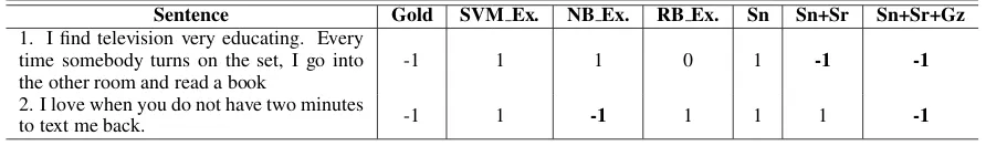
Table 5 shows a few example cases (obtained from test folds) showing the effectiveness of our enhanced feature set.
6 Feasibility of our approach
Since our method requires gaze data from human readers to be available, the methods practicability
becomes questionable. We present our views on this below.
6.1 Availability of Mobile Eye-trackers
Availability of inexpensive embedded eye-trackers on hand-held devices has come close to reality now. This opens avenues to get eye-tracking data from inexpensive mobile devices from a huge population of online readers non-intrusively, and derive cognitive features to be used in predic-tive frameworks like ours. For instance, Co-gisen: (http://www.sencogi.com)has a patent (ID: EP2833308-A1) on “eye-tracking using inexpen-sive mobile web-cams”. Wood and Bulling (2014) have introducedEyeTab, a model-based approach for binocular gaze estimation that runs entirely on tablets.
6.2 Applicability Scenario
We believe, mobile eye-tracking modules could be a part of mobile applications built for e-commerce, online learning, gaming etc. where automatic analysis of online reviews calls for better solutions to detect and handle linguistic nuances in senti-ment analysis setting. To give an example, let’s say a book gets different reviews on Amazon. Our system could watch how readers read the review using mobile eye-trackers, and thereby, decide the polarity of opinion, especially when sentiment is not expressed explicitly (e.g., using strong polar words) in the text. Such an application can hori-zontally scale across the web, helping to improve automatic classification of online reviews.
6.3 Getting Users’ Consent for Eye-tracking
Eye-tracking technology has already been uti-lized by leading mobile technology developers (like Samsung) to facilitate richer user experiences through services likeSmart-scroll(where a user’s eye movement determines whether a page has to be scrolled or not) and Smart-lock (where user’s gaze position decided whether to lock the screen or not). The growing interest of users in us-ing such services takes us to a promisus-ing situa-tion where getting users’ consent to record eye-movement patterns will not be difficult, though it is yet not the current state of affairs.
7 Conclusion
Sentence Gold SVM Ex. NB Ex. RB Ex. Sn Sn+Sr Sn+Sr+Gz
1. I find television very educating. Every time somebody turns on the set, I go into
the other room and read a book -1 1 1 0 1 -1 -1
2. I love when you do not have two minutes
[image:9.595.76.522.63.129.2]to text me back. -1 1 -1 1 1 1 -1
Table 5: Example test-cases from the heldout dataset. Labels Ex→Existing classifier, Sn→Sentiment features, Sr→Sarcasm features and Gz→Gaze features. Values (-1,1,0)→(negative,positive,undefined)
thwarting detection, and (b) cognitive features de-rived from readers’ eye movement behavior. The combined feature set improves the overall accu-racy over the traditional feature set based SA by a margin of3.6%and9.3%respectively for Datasets
1 and2. It is significantly effective for text with complex constructs, leading to an improvement of
6.1% on our held-out data. In future, we pro-pose to explore (a) devising deeper gaze-based features and (b)multi-viewclassification using in-dependent learning from linguistics and cognitive data. We also plan to explore deeper graph and gaze features, and models to learn complex gaze feature representation. Our general approach may be useful in other problems like emotion analy-sis, text summarization and question answering, where textual clues alone do not prove to be suffi-cient.
Acknowledgments
We thank the members of CFILT Lab, especially Jaya Jha and Meghna Singh, and the students of IIT Bombay for their help and support.
References
Apoorv Agarwal, Boyi Xie, Ilia Vovsha, Owen Ram-bow, and Rebecca Passonneau. 2011. Sentiment analysis of twitter data. InProceedings of the Work-shop on Languages in Social Media, pages 30–38. ACL.
Cem Akkaya, Janyce Wiebe, and Rada Mihalcea. 2009. Subjectivity word sense disambiguation. In Proceedings of the 2009 Conference on Empirical Methods in Natural Language Processing: Volume 1-Volume 1, pages 190–199. ACL.
AR Balamurali, Aditya Joshi, and Pushpak Bhat-tacharyya. 2011. Harnessing wordnet senses for supervised sentiment classification. InProceedings of the Conference on Empirical Methods in Natural Language Processing, pages 1081–1091.
Francesco Barbieri, Horacio Saggion, and Francesco Ronzano. 2014. Modelling sarcasm in twitter, a
novel approach. ACL 2014, page 50.
Luciano Barbosa and Junlan Feng. 2010. Robust sen-timent detection on twitter from biased and noisy
data. In Proceedings of the 23rd International
Conference on Computational Linguistics: Posters, pages 36–44. ACL.
Maria Barrett and Anders Søgaard. 2015. Using read-ing behavior to predict grammatical functions. In Proceedings of the Sixth Workshop on Cognitive As-pects of Computational Language Learning, pages 1–5, Lisbon, Portugal, September. Association for Computational Linguistics.
Farah Benamara, Carmine Cesarano, Antonio Pi-cariello, and Venkatramana S Subrahmanian. 2007. Sentiment analysis: Adjectives and adverbs are bet-ter than adjectives alone. InICWSM.
Paula Carvalho, Lu´ıs Sarmento, M´ario J Silva, and Eug´enio De Oliveira. 2009. Clues for detect-ing irony in user-generated contents: oh...!! it’s so easy;-). InProceedings of the 1st international CIKM workshop on Topic-sentiment analysis for mass opinion, pages 53–56. ACM.
Chih-Chung Chang and Chih-Jen Lin. 2011.
LIB-SVM: A library for support vector machines. ACM
Transactions on Intelligent Systems and Technology, 2:27:1–27:27. Software available at http://www. csie.ntu.edu.tw/∼cjlin/libsvm.
Kushal Dave, Steve Lawrence, and David M Pennock. 2003. Mining the peanut gallery: Opinion extraction and semantic classification of product reviews. In Proceedings of the 12th international conference on World Wide Web, pages 519–528. ACM.
C´ıcero Nogueira dos Santos and Maira Gatti. 2014. Deep convolutional neural networks for sentiment analysis of short texts. InProceedings of COLING. Eduard C Dragut and Christiane Fellbaum. 2014. The
role of adverbs in sentiment analysis. ACL 2014,
1929:38–41.
Andrea Esuli and Fabrizio Sebastiani. 2006. Senti-wordnet: A publicly available lexical resource for
opinion mining. InProceedings of LREC, volume 6,
pages 417–422. Citeseer.
Murthy Ganapathibhotla and Bing Liu. 2008. Mining
opinions in comparative sentences. InProceedings
Alec Go, Richa Bhayani, and Lei Huang. 2009. Twit-ter sentiment classification using distant supervision. CS224N Project Report, Stanford, 1:12.
Mark Hall, Eibe Frank, Geoffrey Holmes, Bernhard Pfahringer, Peter Reutemann, and Ian H Witten. 2009. The weka data mining software: an update. ACM SIGKDD explorations newsletter, 11(1):10– 18.
Daisuke Ikeda, Hiroya Takamura, Lev-Arie Ratinov, and Manabu Okumura. 2008. Learning to shift the polarity of words for sentiment classification. In IJCNLP, pages 296–303.
Lifeng Jia, Clement Yu, and Weiyi Meng. 2009. The effect of negation on sentiment analysis and retrieval
effectiveness. InProceedings of the 18th ACM
Con-ference on Information and Knowledge
Manage-ment, CIKM ’09, pages 1827–1830, New York, NY,
USA. ACM.
Salil Joshi, Diptesh Kanojia, and Pushpak Bhat-tacharyya. 2013. More than meets the eye: Study
of human cognition in sense annotation. In
HLT-NAACL, pages 733–738.
Aditya Joshi, Abhijit Mishra, Nivvedan Senthamilsel-van, and Pushpak Bhattacharyya. 2014. Measuring sentiment annotation complexity of text. InACL (2), pages 36–41.
Aditya Joshi, Vinita Sharma, and Pushpak Bhat-tacharyya. 2015. Harnessing context incongruity
for sarcasm detection. Proceedings of 53rd Annual
Meeting of the ACL, Beijing, China, page 757. J Peter Kincaid, Robert P Fishburne Jr, Richard L
Rogers, and Brad S Chissom. 1975. Derivation of new readability formulas (automated readability index, fog count and flesch reading ease formula) for navy enlisted personnel. Technical report, DTIC Document.
Sigrid Klerke, Yoav Goldberg, and Anders Søgaard. 2016. Improving sentence compression by learning
to predict gaze. InProceedings of the 15th Annual
Conference of the North American Chapter of the ACL: HLT. ACL.
Efthymios Kouloumpis, Theresa Wilson, and Johanna Moore. 2011. Twitter sentiment analysis: The good
the bad and the omg! ICWSM, 11:538–541.
Fangtao Li, Minlie Huang, and Xiaoyan Zhu. 2010. Sentiment analysis with global topics and local
de-pendency. InAAAI, volume 10, pages 1371–1376.
Christine Liebrecht, Florian Kunneman, and Antal van den Bosch. 2013. The perfect solution for
detecting sarcasm in tweets# not. WASSA 2013,
page 29.
Chenghua Lin and Yulan He. 2009. Joint
senti-ment/topic model for sentiment analysis. In
Pro-ceedings of the 18th ACM conference on Informa-tion and knowledge management, pages 375–384. ACM.
Bing Liu and Lei Zhang. 2012. A survey of opinion mining and sentiment analysis. InMining text data, pages 415–463. Springer.
Andrew L Maas, Raymond E Daly, Peter T Pham, Dan Huang, Andrew Y Ng, and Christopher Potts. 2011. Learning word vectors for sentiment
analy-sis. InProceedings of the 49th Annual Meeting of
the ACL: Human Language Technologies-Volume 1, pages 142–150. ACL.
Titus Malsburg, Reinhold Kliegl, and Shravan Va-sishth. 2015. Determinants of scanpath regularity in reading. Cognitive science, 39(7):1675–1703. Justin Martineau and Tim Finin. 2009. Delta tfidf:
An improved feature space for sentiment analysis. ICWSM, 9:106.
Diana Maynard and Mark A Greenwood. 2014. Who cares about sarcastic tweets? investigating the
im-pact of sarcasm on sentiment analysis. In
Proceed-ings of LREC.
Qiaozhu Mei, Xu Ling, Matthew Wondra, Hang Su, and ChengXiang Zhai. 2007. Topic sentiment mix-ture: modeling facets and opinions in weblogs. In Proceedings of the 16th international conference on World Wide Web, pages 171–180. ACM.
Abhijit Mishra, Pushpak Bhattacharyya, Michael Carl, and IBC CRITT. 2013. Automatically predicting sentence translation difficulty. In ACL (2), pages 346–351.
Abhijit Mishra, Aditya Joshi, and Pushpak Bhat-tacharyya. 2014. A cognitive study of subjectivity extraction in sentiment annotation. ACL 2014, page 142.
Abhijit Mishra, Diptesh Kanojia, and Pushpak Bhat-tacharyya. 2016. Predicting readers’ sarcasm
un-derstandability by modeling gaze behavior. In
Pro-ceedings of AAAI.
Tony Mullen and Nigel Collier. 2004. Sentiment anal-ysis using support vector machines with diverse
in-formation sources. In EMNLP, volume 4, pages
412–418.
Tetsuji Nakagawa, Kentaro Inui, and Sadao Kuro-hashi. 2010. Dependency tree-based sentiment classification using crfs with hidden variables. In NAACL-HLT, pages 786–794. Association for Com-putational Linguistics.
Vincent Ng, Sajib Dasgupta, and SM Arifin. 2006. Ex-amining the role of linguistic knowledge sources in the automatic identification and classification of
re-views. InProceedings of the COLING/ACL on Main
conference poster sessions, pages 611–618. Associ-ation for ComputAssoci-ational Linguistics.
Bo Pang and Lillian Lee. 2004. A sentimental educa-tion: Sentiment analysis using subjectivity
summa-rization based on minimum cuts. InProceedings of
Bo Pang and Lillian Lee. 2008. Opinion mining and sentiment analysis. Foundations and trends in infor-mation retrieval, 2(1-2):1–135.
Bo Pang, Lillian Lee, and Shivakumar Vaithyanathan. 2002. Thumbs up?: sentiment classification
us-ing machine learnus-ing techniques. InACL-02
con-ference on Empirical methods in natural language processing-Volume 10, pages 79–86. ACL.
Raja Parasuraman and Matthew Rizzo. 2006.
Neuroer-gonomics: The brain at work. Oxford University Press.
Kashyap Popat, Balamurali Andiyakkal Rajendran, Pushpak Bhattacharyya, and Gholamreza Haffari. 2013. The haves and the have-nots: Leveraging
unlabelled corpora for sentiment analysis. InACL
2013 (Hinrich Schuetze 04 August 2013 to 09 Au-gust 2013), pages 412–422. ACL.
Soujanya Poria, Erik Cambria, Gregoire Winterstein, and Guang-Bin Huang. 2014. Sentic patterns: Dependency-based rules for concept-level sentiment
analysis. Knowledge-Based Systems, 69:45–63.
Ankit Ramteke, Akshat Malu, Pushpak Bhattacharyya, and J Saketha Nath. 2013. Detecting turnarounds in sentiment analysis: Thwarting. InACL (2), pages 860–865.
Keith Rayner and Susan A Duffy. 1986. Lexical com-plexity and fixation times in reading: Effects of word frequency, verb complexity, and lexical ambiguity. Memory & Cognition, 14(3):191–201.
Keith Rayner and Sara C Sereno. 1994. Eye move-ments in reading: Psycholinguistic studies.
Ellen Riloff, Ashequl Qadir, Prafulla Surve, Lalin-dra De Silva, Nathan Gilbert, and Ruihong Huang. 2013. Sarcasm as contrast between a positive
senti-ment and negative situation. InEMNLP, pages 704–
714.
Hassan Saif, Yulan He, and Harith Alani. 2012. Al-leviating data sparsity for twitter sentiment analysis. CEUR Workshop Proceedings (CEUR-WS. org).
Raksha Sharma and Pushpak Bhattacharyya. 2013.
Detecting domain dedicated polar words. In
Pro-ceedings of the International Joint Conference on Natural Language Processing.
Titus von der Malsburg and Shravan Vasishth. 2011. What is the scanpath signature of syntactic reanaly-sis? Journal of Memory and Language, 65(2):109– 127.
Janyce Wiebe and Rada Mihalcea. 2006. Word sense and subjectivity. InInternational Conference on Computational Linguistics and the 44th annual meeting of the ACL, pages 1065–1072. ACL.
Theresa Wilson, Janyce Wiebe, and Paul Hoffmann. 2005. Recognizing contextual polarity in
phrase-level sentiment analysis. In EMNLP-HLT, pages
347–354. Association for Computational Linguis-tics.
Erroll Wood and Andreas Bulling. 2014. Eyetab: Model-based gaze estimation on unmodified tablet
computers. InProceedings of the Symposium on Eye