Assessing the Quality of Spot Welding Electrode
Tips Using Image Processing Techniques
Abdulwanis Abdulhadi, Munther Gdeisat, Dave Burton, and Francis Lilley
Abstract— Spot welding is used extensively in the
automotive industry. The quality of an individual welding spot is a major concern due to the heavy reliance on their use in the manufacture of cars. The main parameters that control the quality of a welding spot are current, voltage, welding force, welding time, and the quality of the welding electrodes. The condition of the welding electrodes plays a major part in determining the quality of a welding spot. For example, excessive wear can occur during the welding process and can cause weakening in the weld nuggets. As the number of welds increases, the electrode tip wears down and so the contact area between electrode tip and work piece increases. Hence the applied current should be increased in order to maintain the same current density so as to preserve the quality of the welding nuggets. In order to determine the quality of the welding electrodes, images of the electrode tips are captured and are processed using various image-processing algorithms. These algorithms can be used to measure the tip width and hence assess the quality of the electrodes. The quality of two types of spot welding electrode tips, dome and flat tips, is assessed using image processing and boundary representation techniques. For each tip type, a database of 250 images is used to test the performance of our algorithms. Also the quality of the tip for these 250 images is determined manually. An excellent agreement is found between these manual and automatic methods.
Index Terms—Spot welding, image segmentation,
boundary representation
I. INTRODUCTION
ESISTANCE spot welding (sometimes referred to as “resistance welding”) is a quick and easy way of joining two materials [1], [2]. The most common application of resistance spot welding is in the automotive industry as it lends itself to rapid, high-volume welding applications, of which this is a prime example. It can be used to join together two or more metallic worksheets. This is achieved by means of the welding electrodes, which are placed into forcible contact on either side of the work pieces that are to be joined, and then by passing electrical current through both the electrodes and the stacked sheets in order to generate heat and cause fusion at the faying interface of the worksheets. Each weld sequence consists of four main stages: 1) clamping of the work piece; 2) applying the weld force required for welding [3], [4]; 3) applying the weld current that is necessary for fusion of the work pieces [5], [6]; 4) a final retraction of the electrodes after the molten nugget has solidified. This process is illustrated in Figure 1.
Manuscript received March 6, 2011; revised March 29, 2011. The authors are with The General Engineering Research Institute (GERI), Liverpool John Moores University, James Parsons Building,
When melting has occurred, the current is removed and the original pressure is held for a short period of time thereby allowing the metals to solidify. At this point the weld ‘’nugget’’ is formed. This nugget is the point at which the two metals are joined together and the volume of this joint is of paramount importance to the final strength of the weld. If this nugget is too small then the weld is likely to be weak and the risk of the two metals separating during use is significantly increased. An important factor in determining the size of the weld nugget is the surface area of the electrodes at the point of contact.
Fig. 1. How weld nuggets are formed.
Degradation of the electrode tips results in a loss of their ability to perform their functions. The three functions of a resistance welding electrode are to provide the necessary weld force, weld current density, and cooling. Typical electrode degradation occurs when the tip diameter of the electrode grows too large to convey adequate current density to the work piece. This process is illustrated in Figure 2. As the diameter of the tip (tip width Tp) increases, so does the surface
area of the tip. This results in a reduced current density and means that the heat generated during the welding process is insufficient, hence resulting in a smaller weld nugget [7], [8].
In this paper, we propose using image processing algorithms to automatically determine the tip width. Firstly, we capture an image of the electrode. Then we use an image segmentation algorithm such as the snake active contours method to extract the electrode from the image [12]-[18]. The boundary of the electrode object within the segmented image is then determined. This boundary is filtered using for example, the Fourier transform boundary descriptor algorithm, or minimum perimeter polygon methods [9]. Finally, the tip width is extracted from the filtered boundary.
p
T
p
C
Fig. 2. (a) new electrode dome tip, (b) worn electrode tip.
II. FINDINGTIPWIDTH
Firstly, we shall introduce Cullen et al.’s method to automatically determine the tip width [8]. Figure 3 shows an image that contains a flat tip and indicates its parameters such as the tip width Tp and the electrode
width Cp. Figure 4 shows a schematic diagram of an
[image:2.595.326.548.71.220.2]ideal flat tip.
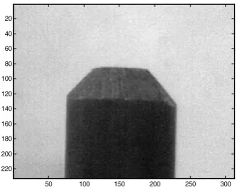
[image:2.595.58.280.74.171.2]Fig. 3. An image showing a real flat tip.
Fig. 4. A schematic diagram of an ideal tip.
Figure 5 shows an image that contains the boundary of the ideal flat tip.
Fig. 5. An image showing the boundary of the tip and tip parameters.
Suppose that the size of both the tip image and the boundary image are M × N pixels. Let us process the boundary image on a row by row basis. For each row, we subtract the x coordinates of the left boundary
points (shown in red colour) from the x coordinates of
the right boundary points (shown in blue colour). The first xa rows (see Fig. 5) do not contain the tip
boundary. The subtraction operation produces zeros as shown in Figure 6. For the row xa +1, the subtraction
operation produces the tip width Tp. For the rows from
xa + 1 until xa + xg, the subtraction operation produces a
line with a slope of
2
2 tan
p p gg g
C
T
y
g
x
x
θ
−
=
=
=
(1)The value of θ can be determined by measuring the slope angle of the tip under inspection, or extracted from the manufacturer’s datasheet. Similarly, the value of the electrode width Cp can be either measured, or
extracted from the manufacturer’s datasheet. For the tip that is shown in Figure 3, the tip slope angle is close to 45o.
For the rows from xa + xg + 1 until M, the subtraction
operation produces a value of Cp. The results of the
[image:2.595.73.240.309.442.2]subtraction operation are indicated in the 2D graph that is shown in Figure 6.
Fig. 6. The profile of the tip.
50 100 150 200 250 300
20
40 60
80
100
120 140
160
180
200 220
x
y
a
x
pT
pC
a g
x
+
x
M
x
y
(0,0)
p
T
g
y
g
x
p
C
θ
a
x
image
borders
(M−1,N−1)
p
T
p
T
( )
a
( )
b
x
y
(0,0)
p
T
p
[image:2.595.84.228.484.613.2] [image:2.595.324.532.590.726.2]The first derivative of the 2D graph in Figure 6 is calculated and this is shown in Figure 7.
[image:3.595.63.273.105.210.2]Fig. 7. The first derivative of the tip profile shown in Figure 6.
The width of the tip is determined as follows. The derivative of the tip profile is thresholded using a threshold value g. The value of the tip gradient g is
known a priori. Then the number of points whose
values are larger than g is determined and this number
is assigned to xg. The tip width is then determined
using Equation (1).
[image:3.595.324.522.106.261.2]The following example explains the process of determining the width of the tip using a real image. The image shown in Figure 3 is processed in order to extract the electrode from the image using an image processing algorithm. Then the boundary of the tip is outlined as shown in Figure 8. After that the profile of the tip is calculated by subtracting the left-hand boundary of the tip from the right-hand boundary. The profile of the tip is shown in Figure 9.
Fig. 8. The boundary of the real tip that was shown in Figure 3.
Fig. 9. The profile of the tip that was shown in Figure 3.
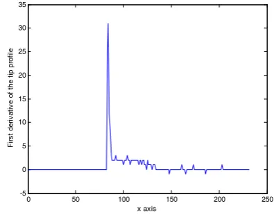
The first derivative for the tip profile is then calculated and this is illustrated in Figure 10.
Fig. 10. The first derivative of the tip profile shown in Figure 9.
The first derivative mathematical operation amplifies the noise in the tip profile and this complicates the process of extracting the tip width Tp. For example, the
tip width for the electrode that is shown in Figure 3 is approximately 60 pixels. The maximum value of the first derivative should be close to Tp. However, this
maximum value is 31. This large error is introduced mainly by noise. Hence, it is not possible to use this maximum value to determine the tip width. This indicates the necessity to filter the tip profile before calculating the first derivative.
For the electrode that is shown in Figure 3, the value of g is equal to 2. xg is found to be equal to 49. Cp is
[image:3.595.66.224.420.543.2]equal to 156 and this is determined directly from Figure 9 by calculating the maximum value of the tip profile. The tip width is then calculated as being 58 pixels.
III. IMAGEPROCESSING
To determine the tip width from the tip image, it is necessary to produce an outline of the tip. This task can be carried out by separating the electrode in the image from the image background and this procedure can be carried out by using image segmentation techniques. This can be a difficult task to perform due to the presence of noise, other objects in the image, non-uniform background illumination, and specular reflections in the electrode. We have carried out exhaustive research in order to find an algorithm to successfully extract the electrode in the image that is shown in Figure 2(a) [9]. Many image segmentation algorithms failed, but we found that the snake active contours algorithm can adequately fulfil the segmentation task. We tested the snake algorithm using 250 images and it has successfully segmented them all [12].
As explained above, the first derivative of the tip profile is noisy. To reduce these noise effects, the tip profile should be filtered before applying the derivative operation. We have used two methods here to filter the Pixels
P
ix
els
50 100 150 200 250 300
20 40 60 80 100 120 140 160 180 200 220
0 50 100 150 200 250
0 20 40 60 80 100 120 140 160
x axis
Ti
p pr
of
ile
0 50 100 150 200 250
-5 0 5 10 15 20 25 30 35
x axis
Fi
rs
t der
iv
at
iv
e of
t
he t
ip pr
of
ile
x
ax
pT
a g
x
+
x
M
g
y
[image:3.595.65.262.589.742.2]tip profile: namely the Fourier transform and the minimum perimeter polygon approaches.
[image:4.595.68.270.225.406.2]Figure 11 shows three different combinations of the image segmentation and image representation algorithms that may be used to extract the tip width. The first combination uses the snake active contours algorithm and Cullen et al.’s method. The second combination uses the snake active contours algorithm, the Fourier transform approach and Cullen et al.’s method. The third combination uses the snake active contours algorithm, the minimum perimeter polygon algorithm and Cullen et al.’s method.
Fig. 11. Image segmentation and boundary representation and description.
A. Snakes active contour and Cullen methods
Snakes are curves that are defined within the image domain that can move under the influence of internal forces coming from within the curve itself and also from external forces computed from the image data. The internal and external forces define the snakes and will conform to an object’s boundary, or to other desired features within an image. Snakes are widely used in many applications, including edge detection [12], shape modelling [13, 14], segmentation [15, 16], and motion tracking[17, 18]. In this paper, we use parametric active contours within an image domain and allow them to move toward desired features, usually edges.
There are two key difficulties with parametric active contour algorithms. First, the initial contour must, in general, be close to the true boundary, or else it will be likely converge to the wrong result. The second problem is that active contours have difficulties progressing into boundary concavities [17, 18].
A traditional snake is a curve defined by
],
1
,
0
[
)],
(
),
(
[
)
(
s
=
x
s
y
s
s
∈
x
that moves through thespatial domain of an image to minimize the energy function
[
x s x s]
x s dsE
E
ext( ( )) )
( )
( 2 1
1
0
2 '' 2
' + +
=
∫
α β (2)Where α and β are weighting parameters that control the snake’s tension and rigidity, respectively, and the terms
x
'(x) andx
''(s) respectively denote the first andsecond derivatives of
x
(
s
)
with respect to s. Theexternal energy function Eextis derived from the image
so that it takes on its smaller values at features of interest, such as boundaries.
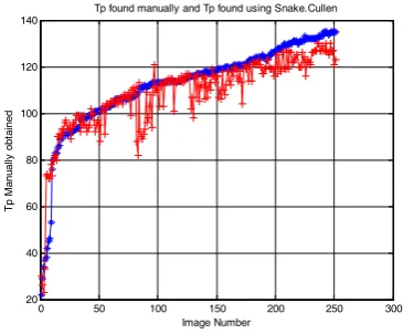
We have used the snake active contour method to segment 250 images and to determine the boundary of the electrode in these images. The segmented images are then applied to Cullen et al.’s method for estimating the tip width. The results are shown in Figure 12 using the red colour trace.
[image:4.595.332.515.292.443.2]In order to assess the performance of the above algorithm, we also manually measured the tip width for the 250 images and the results are shown in Figure 12 using the blue colour trace.
Fig. 12. Determining the tip width manually (shown in blue colour) and automatically using snake active contour and Cullen et al.’s methods (shown in red).
Fig. 13. The error between estimating the tip width manually and automatically using snake active contours and Cullen et al. methods.
B. Snakes active contour, Fourier transform
boundary descriptor and Cullen methods
The boundary shown in Figure 8 can be filtered using a Fourier transform boundary descriptor method as explained here. Figure 8 shows a K-point digital
boundary in the xy plane. Starting at an arbitrary point
(xo, yo), coordinate pairs (xo, yo), (x1, y1), (x2, y2),..., (x
K-0 50 100 150 200 250 300
20 40 60 80 100 120 140
Image Number
Tp M
anual
ly
obt
ai
ned
Tp found manually and Tp found using Snake.Cullen
0 50 100 150 200 250 300
-40 -30 -20 -10 0 10 20
30 Error between Tp found manually and Tp found using Snake.Cullen
Image Number
Tp E
rror
obt
ained
Electrode
image Snake active contours algorithm
Cullen et al. algorithm
Fourier
transform Cullen et al. algorithm
Minimum perimeter polygon method
Cullen et al. algorithm
Image segmentation
[image:4.595.325.531.500.628.2]1, yK-1) are encountered in traversing the boundary in a
counter clockwise direction. These coordinates can be expressed in the form x(k) = xk and y(k) = yk. With this
notation, the boundary itself can be represented as the sequence of coordinates s(k) = [x(k), y(k)], for k = 0, 1,
2, K-1. Moreover, each coordinate pair can be treated
as a complex number as s(k) = x(k)+iy(k). That is the x
axis is treated as the real axis, and the y axis as the
imaginary axis of a sequence of complex numbers. The discrete Fourier transform of s(k) is
(3)
For u = 0, 1, 2, .... , K-1. The complex coefficients a(u) are called the Fourier descriptors of the boundary.
The inverse Fourier transform of these coefficients restores s(k). That is,
(4)
For u = 0, 1, 2, K-1. Suppose, however, that instead
of all the Fourier coefficients, only the first P
coefficients are used. This is equivalent to setting the term a(u) = 0 for u > P-1. Then we get an
approximation for the boundary. The low frequency components account for the global shape of the boundary, whereas the high frequency components account for the fine details in the boundary shape.
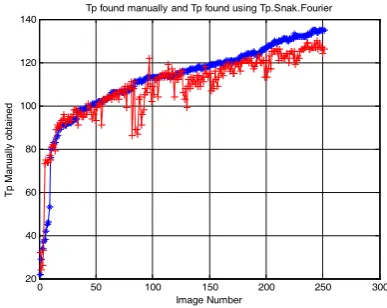
As explained previously, in the second combination of techniques, the electrode in the 250 images is extracted using the snake active contour method. Also, this method determines the boundary of the electrode. The boundary is then filtered using the Fourier transform boundary descriptor method. P is set here to
a value of 110. The filtered boundary is then applied to Cullen et al.’s method for determining the tip width. The results are shown in Figure 14 using the red colour trace. The tip width is also extracted manually and the results are shown using the blue colour trace. The mathematical differences between the results that were produced manually and those that were produced using this automatic method are shown in Figure 15.
C. Snakes active contour , minimum perimeter
polygon and Cullen methods
[image:5.595.326.520.76.230.2]Figure 8 shows a boundary that can be approximated with arbitrary accuracy by a polygon. For a closed boundary, the approximation becomes exact when the number of vertices of the polygon is equal to the number of points in the boundary, and each vertex coincides with a point on the boundary. The details and the noise in the boundary can be reduced by decreasing the number of vertices.
Fig. 14. Determining the tip width manually (shown in blue colour) and automatically using the snake active contour, Fourier transform
[image:5.595.328.521.290.424.2]boundary descriptor and Cullen et al.’s methods (shown in red).
Fig. 15. The error between estimating the tip width manually and automatically using the snake active contours, Fourier transform
boundary descriptor and Cullen et al.’s methods.
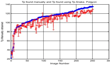
As explained previously, in the third combination the electrode in the 250 images is extracted using the snake active contour method. The boundary is then filtered using the minimum perimeter polygon algorithm [9]. The cell size is set here to a value of 2 and this results in a low resolution boundary with much of the noise removed. The filtered boundary is then applied to Cullen et al.’s method to determine the tip width. The results are shown in Figure 16 using the red colour trace. The tip width is also extracted manually and the results are shown using the blue colour trace. The mathematical differences between the results that were produced manually and those that were produced using this automatic method are shown in Figure 17.
We have calculated the respective standard deviations for the errors that are shown in Figures 13, 15 & 17. The results are shown in the table below. The results in this table reveal that the specific combination of the snake algorithm, Fourier transform boundary descriptor approach and Cullen et al.’s method gave the most accurate automatic estimation for the tip width. On the other hand, the specifc combination of the snake algorithm and Cullen et al.’s method produces the worst automatic estimation results for the tip width.
0 50 100 150 200 250 300
20 40 60 80 100 120 140
Image Number
Tp M
anual
ly
obt
ai
ned
Tp found manually and Tp found using Tp.Snak.Fourier
0 50 100 150 200 250 300
-20 -10 0 10 20 30 40 50
60 Error between Tp found manually and Tp found using Tp.Snak.Fourier
Image Number
Tp E
rror
obt
ai
ned
1 2 /
0
( )
K( )
j uk Kk
a u
s k
e
π− −
=
=
∑
1
2 /
0
1
( )
K( )
j uk Ku
s k
a u
k
e
π −
=
Fig. 16. Determining the tip width manually (shown in blue colour) and automatically using snake active contour, minimum perimeter polygon and Cullen et al.’s methods (shown in red).
Fig. 17. The error between estimating the tip width manually and automatically using snake active contours, minimum perimeter polygon and Cullen et al.’s methods.
TABLEI
STANDARD DEVIATION FOR THE THREE COMBINATIONS
IV. CONCLUSION
This paper has shown that it is possible to perform the analysis of the spot welding electrode tip automatically. This can be used to determine when to redress the electrode tip. This method of performing the tip width analysis has been carried out on a tapered tip, but works equally well for analysing tips that are domed in shape. All the algorithms work well with a set of two hundred and fifty images that we have produced experimentally. Our study reveals that the approach combining the snake active contours algorithm, the Fourier transform boundary descriptor
approach and Cullen et al.’s method gives the best automatic estimation results for the tip width.
REFERENCES
[1] X. Sun, ’’Effect of projection height on projection collapse and nugget formation-finite element study’’ Welding Journal, pp.
211-s-216-s, Sept. 2001.
[2] H. D. Orts, “The Effects of Tic composite coating in resistance spot welding Galvanized Steel”, Master Thesis, Ohio State University, USA, 1967.
[3] C. SM Nealon and L. S. H. Lake, ”Resistance spot welding tip lives for zincalume coated qualities’’, BHP steel research and technology centre, research report no. 950, January 1987. [4] R. W. Jud, ’’Joining Galvanised and galvanneal steels’’, SAE
Technical paper series, No 840285, 1984.
[5] A. Morita, S. Inour and A. Takezoe ’’Spot weldability of zinc vapour deposited steel sheets’’, Journal of metal finishing society, Japan. vol. 39, No. 5, pp.270-275.
[6] L. M. Friedman and R. B. McCauley, “Influence of metallurgical characteristics on resistance welding of Galvanized steel”, Welding Journal, Supplement, pp. 454-462s,
Oct.1969.
[7] T. Saito, ’’Resistance weldability of coated sheet for automotive application’’, Journal Welding International, vol.6,
No.9, pp. 695-699, 1992.
[8] A. Mason, J. D. Cullen, A. I. AI-Shmma’a and W. Lucas, ‘’ Real time image processing of electrode profilein resistance spot welding,’’ Journal of Physics: Conference Series, ISSN:
1742-6588, vol. 15, pp. 336-3441, 2005.
[9] R. C. Gonzalez, R. E. Woods and S. L. Eddins Digital Image Processing using MATLAB, 2004.
[10] J. D. Cullen, N. Athi, M. Jader, P. Johnson, A. I. AL-Shamma,a, A. Shaw and A. M. A. EL-Rasheed, ‘’Multisensor fusion for on line monitoring of the quality of spot welding in automotive industry‘’, Measurement, vol 41, Issue 4, pp.
412-423, 2008.
[11] D. Cullen, N. Athi, A. M. Jader, A. Shaw, and A. Al-Shamma’a, “Energy reduction for the spot welding process in the automotive industry”, Sensors And Their Applications XIV Conference (SENSORS07), Liverpool, UK, 11–13 September
2007, Journal of Physics: Conference Series, ISSN: 1742-6588, Vol. 76, IOP Publishing, Article No. 012022, 2007.
[12] M. Kass, A. Witkin, and D. Terzopoulos, “Snakes: Active contour models,” Int. J. Comput. Vis., vol. 1, pp. 321-331,1987.
[13] D. Terzopoulos and K. Fleischer, “Deformable models,” Vis Comput., vol. 4, pp. 306-331, 1988.
[14] T. McInerney and D. Terzopoulos, ”A dynamic finite element surface mode for segmentation and tracking in multidimensional medical images with application to cardiac 4D image analysis,” Comput. Med. Imag. Graph., vol. 19, pp.
69-83, 1995.
[15] F. Leymarie and M. D. Levine, “Tracking deformable objects in the plane using an active contour model,” IEEE Trans. Pattern Anal. Machine Intell., vol. 15, pp. 617-634, 1993.
[16] R. Durikovic, K. Kaneda and H. Yamashita,” Dynamic contour: A texture approach and contour operations, “ Vis. Comput., vol.
11, pp. 277-289,1995.
[17] D. Terzopoulos and R. Szeliski, ”Tracking with Kalman snakes,” in Active Vision, A. Blake and A. Yuille, Eds.
Cambridge, MA: MIT press, 1992, pp. 3-20.
[18] V. Caselles, F. Catte, T. Coll and F. Dibos, “A geometric model for active contours,” Numer. Math., vol. 66, pp. 1-31,1993.
0 50 100 150 200 250 300
20 40 60 80 100 120 140
Image Number
Tp M
anual
ly obt
ained
Tp found manually and Tp found using Tp.Snake. Polgyon
0 50 100 150 200 250 300
-30 -20 -10 0 10 20 30
40Error between Tp found manually and Tp found using Tp .Snake. Polgyon
Image Number
Tp E
rror
obt
ained
Combination standard
deviation Snake active contour and Cullen et al.’s
method. 7.3
Snake active contour, Fourier transform boundary descriptor and Cullen et al.’s method.
6.8