Risk-adjusted Joint Optimization of Base-stock
Levels and Component Allocation in an ATO
System with Returns
Ebru Ang¨un, Eda Bilici
Abstract—We consider a multi-component, multi-product, periodic-review (re)assemble-to-order (RATO) system that uses an independent base-stock policy for the inventory replenish-ment of the components. At the beginning of each period, end-of-lease cores are returned. Because the quality of cores is random, they are tested, graded, and sorted into four pre-specified quality levels. Then, the random, jointly and continuously distributed demands for the products are realized. In our problem, partial fulfillment is not allowed. Furthermore, the system quotes a predetermined response time window for each product, and it penalizes the system if the demand is not satisfied within its time window. We model this problem through a risk-adjusted two-stage stochastic programming problem, where the first-stage decisions are the base-stock levels for all components, and the second-stage decisions are the allocations of components to different products. The risk adjustment is formulated through a chance constraint, which is then replaced by a conditional value-at-risk constraint. We solve the resulting problem through the sample average approximation method combined with the L-shaped method. We also present some encouraging numerical results.
Index Terms—Monte Carlo simulation, reverse logistics, risk measures, stochastic programming.
I. INTRODUCTION
P
RODUCT recovery can be performed in many ways such as remanufacturing, reconditioning, recycling, can-nibalizing and refurbishing of products. The reuse of product returns (also called cores) can be very profitable, especially for the high-tech products that have quite long product life cycles. For instance, the characteristic life cycle of a computer chip is 80,000 hours for which only 20,000 hours are used; therefore, that chip can still be economically used for 60,000 hours in some other products through, say, remanufacturing; see Geyer et al. (2007). Remanufacturing is one of the highly important field of product recovery. In the context of our paper, it refers to the process through which a core is brought to an as good as new condition by inspecting its components, and performing repairing, replacing, restoring operations and/or updating it with new specifications when necessary. This operation is widely found for high-valued industrial products like photocopiers, com-puters, cellular phones, aviation equipments, vehicle engines, and telecommunication or medical equipments.Many firms have been looking for ways to decrease their response times to the market because the pressure for serving
Manuscript received December 31, 2011; revised January 12, 2012. This research has been financially supported by Galatasaray University Research Fund.
E. Ang¨un is with the Department of Industrial Engineering, Galatasaray University, Istanbul, 34357 TURKEY (e-mail: [email protected]).
E. Bilici is with the Department of Industrial Engineering, Galatasaray University, Istanbul, 34357 TURKEY (e-mail: [email protected]).
customers speedily and the impacts of product obsolescence increase. One way to deal with the aforementioned issues is to adopt an assemble-to-order (ATO) manufacturing strat-egy and/or its variations (i.e., reassemble-to-order (RATO), configure-to-order, etc.) instead of employing the traditional make-to-stock system. In an (R)ATO system, the inventories are held at component or part levels, which substantially reduces the inventory holding costs. This (R)ATO system further increases customer satisfaction through decreasing response times to the demands and increasing fill rates (i.e., the fraction of demands satisfied from on-hand inventory to the total demands).
Our paper contributes to the existing literature in the following ways:
• This paper considers the joint optimization of the base-stock levels and component allocation in case there are cores of uncertain quality.
• The problem is considered in a risk-adjusted manner by considering the so-called conditional-value-at-risk constraint.
The first item was also considered in Akc¸ay and Xu (2004), but in a risk-neutral environment and without remanufactur-ing.
The rest of the paper is organized as follows. In Section 2, we present a description of the system, and in Section 3 we present the risk-adjusted two-stage optimization problem. In Section 4, we present our numerical results, and in Section 5 our conclusions and future research.
II. SYSTEMDESCRIPTION
We consider a hybrid assemble-to-order (ATO) and reassemble-to-order (RATO) system with m components, indexed by i = 1, ..., m, and n products, indexed by
j = 1, ..., n. The following sequence of events is typical for the system for every period t, t = 0,1,2, .... At the beginning of a period, the inventory position (i.e., on-hand inventory plus on-order inventory minus backorders) of each component is reviewed, and the component replenishment orders are placed according to the inventory policy. After the receipt of the replenishment for earlier orders and update of the inventory positions of the components, end-of-lease products (cores) are returned. These cores are subject to be tested, graded, and sorted into a number of quality levels, so that the random amounts of cores which fall into each quality level are revealed. Then, random orders for different products arrive through lease agreements.
component i denoted by Si. The replenishment lead time
of componenti, denoted byLi, is deterministic and integer,
which is an integer multiple of the review interval. These lead times can be different for different components.
The return time and quantity of the cores are considered as deterministic. However, the quality of the cores is difficult to predict. Hence, they are tested, graded, and sorted into four quality levels; see the Xerox Europe case study in [6]. The cores of quality level 1 (i.e., best cores) require only refurbishing, and the cores of quality level 2 can be remanufactured. Moreover, the cores of quality level 3 are disassembled, and after being repaired, some of their com-ponents enter the inventories of the brand-new comcom-ponents. Finally, the cores of quality level 4 are immediately disposed off at negligible costs.
In this study, we assume no market segmentation between remanufactured and manufactured products. Each manufac-tured (brand-new) product is assembled from multiple units of a subset of m components, and each core of quality level 2 is remanufactured by replacing a prespecified number of components. Let bij and b0ij2 denote the usage rates
of component i to manufacture and to remanufacture unit demand of product j, respectively, where bij ≥ b0ij2. The
system quotes a response time window, wj, for product j.
This time window is prespecified and fixed for every product type by the system. We assume that the system is penalized by a unit penalty, qj, if a demand for product j cannot
be filled within wj periods after its arrival. Furthermore, a
demand for productjis considered to be filled if that demand is allocated bij or b0ij2 units of component i (no partial
shipment is allowed). All unfilled demands are completely backlogged. The system uses the following order to fill the demands: first, the cores of quality level 1, then the cores of quality level 2, and finally the manufactured products. This order is reasonable because the production times and component requirements increase in the same order.
The problem of interest is analyzed in two stages. The first-stage decisions are the optimal base-stock levelsSi for
i= 1, ..., m, and these decisions are taken without observing the realizations of the random amounts of cores of different quality levels and the realizations of the random demands for the n products. After the cores are tested and graded, and customers’ demands are received, the second-stage decisions, namely the amounts of inventories to be allocated to the unfilled demands, are made in each period. We assume that the inventories are allocated to the unfilled demands subject to a first-come first-served (FCFS) inventory commitment rule. Under the FCFS rule, no inventory is allocated to the demands received in later periods unless earlier backlogs for a component are completely satisfied. The FCFS rule has been adopted by [1], [2], and [8].
Now, we introduce new random variables, which depend on the joint random demands (P1t, P2t, ..., Pnt) for the
n products and the joint random amounts of the cores that fall into four quality levels (Rjt1, Rjt2, Rjt3, Rjt4)for
j = 1, ..., n and t = 0,1, .... These new random variables will be used to derive an equation for the inventory on-hand. Let Dit and Qit be the total demand for component i in
period t and the total amount of component idisassembled from cores of quality level 3, respectively, for i= 1, ..., m.
Then,
Dit= n
X
j=1
h
b0ij2minn(Pjt−Rjt1) +
, Rjt2
o
+bij(Pjt−Rjt1−Rjt2)
+i
Qit= n
X
j=1
b0ij3Rjt3
where, for any two random variablesXandY,(X−Y)+= max{X−Y,0}. We further denote the amount of replenish-ment for componentiin periodtand the net inventory level (i.e., on-hand inventory minus backlog) of component i at the end of periodtbyAitandIit, respectively. LetDi[s, t],
Ai[s, t], and Qi[s, t] be the total demand, the total
replen-ishment, and the total disassembled amount for componenti
from periodsthrough periodtinclusive, respectively, where
Di[s, t] = t
X
u=s
Diu Ai[s, t] = t
X
u=s
Aiu
Qi[s, t] = t
X
u=s
Qiu.
Now, we derive an equation for the inventory on-hand. Assume that k is a nonnegative integer such that k ≤ Li
for any lead time Li. Because each component is operated
under an independent base-stock levelSi, based on [7], the
following equation for the net inventory level at the end of periodt+kcan be written for i= 1, ..., m
Ii,t+k=Si−Di[t+k−Li, t+k]
+Qi[t+k−Li, t+k].
(1)
Furthermore, using balance equations and FCFS inventory commitment rule, the net inventory level at the end of period
t+kis related to the one at the end of periodt−1as follows
Ii,t+k=Ii,t−1+Ai[t, t+k]−Di[t, t+k]
+Qi[t, t+k].
(2)
Substituting (2) in (1), we reach the following result
Ii,t−1+Ai[t, t+k] +Qi[t, t+k] =
Si−Di[t+k−Li, t−1] +Qi[t+k−Li, t+k]. (3)
Note that Ii,t−1 + Ai[t, t+k] + Qi[t, t+k] is the net
inventory level at the end of period t +k after having received all replenishment orders and having disassembled all repairable componentsifrom cores of quality level 3, but before allocating any inventory to the demands realized after periodt−1. Furthermore, because of the FCFS rule, if the amount Si−Di[t+k−Li, t−1] +Qi[t+k−Li, t+k]
is positive, that inventory will be committed to the demands
(P1t, P2t, ..., Pnt) of period t before any demands of the
subsequent periods. Now, suppose that the response time windows for then products can be ordered as w1 ≤w2 ≤
...≤wn. Then, the on-hand inventory of componentito be
committed to(P1t, P2t, ..., Pnt)for k= 0,1, ..., wn is given
by
(Si−Di[t+k−Li, t−1]
+Qi[t+k−Li, t+k])+.
Before presenting the formulation, we assume the follow-ing: the longest response window wn does not exceed the
shortest of the lead timesLi; i.e.,wn≤ min
1≤i≤mLi. This is a
plausible assumption because if there exists any productjfor which the lead time of component i satisfies Li < wj, that
componentican be replenished to fill the orders of productj
before its response time windowwj. Hence, the componenti
will not be considered in the allocation problem for product
j.
In the following, for ease of exposition, we shall focus on stationary random data so that the on-hand inventory level of component iin (4) becomes
(Si−Di[Li−k] +Qi[Li+ 1])+. (5)
III. RISK-ADJUSTEDTWO-STAGESTOCHASTIC PROGRAMMINGFORMULATION
We consider the following problem with a chance con-straint:
min
S=(S1,...,Sm)T∈Rm
cTS+E[Q(S,ε)]
s.t. Prob{Q(S,ε)≤η} ≥1−α
S≥Ssafe
(6)
where for a realizationεe=Pe1, ...,Pen,Re11, ...,Ren4
of ε, the second-stage costQ(S,εe)is given by
min qTu
s.t.
n
P
j=1
k
P
l=0
b0ij2xrjl+bijxmjl
≤
Si−Dei[Li−k] +Qei[Li+ 1]
+
(7a)
for k= 0,1, ..., wn andi= 1, ..., m wj
P
l=0
xr jl+x
m jl
+uj=
e
Pj−Rej1
+
(7b)
for j= 1, ..., n
wj P
l=0
xr
jl≤Rej2 forj = 1, ..., n (7c)
xrjl≥0, xmjl ≥0, uj ≥0
forl= 0, ..., wj andj= 1, ..., n.
In the following, we define the notation in (6) and (7). c= (c1, ..., cm)
T
is vector of procurement costs per unit of themcomponents,S= (S1, ..., Sm)
T
is vector of base-stock levels of themcomponents,Ssafe= (S1s, ..., Sms)
T
is vector of mean safety stock levels for the m components during their lead times, η is upper bound on random second-stage cost Q(S,ε), and αis significance level where α∈(0,1). The first-stage here-and-now decisions are the base-stock levels (S1, ..., Sm), and these decisions are made before
observing the random data. Furthermore, q= (q1, ..., qn) T
is vector of shortage costs per unit of the n products, and u = (u1, ..., un)T is vector of shortage amounts of the n
products. The second-stage wait-and-see decisions are the remanufactured and manufactured amounts xr
jl and xmjl of
product j (j = 1, ..., n), respectively, within its response time window l = 0,1, ..., wj, and the shortage amounts
uj. The second-stage decisions are made after observing the
random demands and the random amounts of cores that fall into each of the four quality levels. Moreover, (7a) implies that the amount of component i used for remanufacturing
and manufacturing within response time windows cannot exceed its on-hand inventory level; (7b) implies that the total remanufactured and manufactured amounts of productj
within its response time windowwjplus the shortage amount
has to be equal to the net demand
e
Pj−Rej1
+
for product
j, because the cores of quality level 1 (i.e.,Rej1) are ready to
fill the demand for productjafter only minor servicing. Fur-thermore, (7c) implies that the total remanufactured amounts of productj within wj cannot exceed the remanufacturable
amountRej2 for product j. Additionally, in case all penalty
costs areqj= 1, the objective function in (7) divided by the
sum of the expected demands for alln products equals the expected average no-fill rate (i.e., the complement of fill rate with respect to one).
The formulation (6) provides a risk-adjusted approach to the problem; i.e., it minimizes the random second-stage costQ(S,ε)on average, while controlling its upper limitη
for different realizations of the random data. A well-known problem of such a formulation is that chance constraints usually define non-convex feasible sets. It was suggested in [9] to replace chance constraints by conditional value-at-risk constraints, where the Conditional Value-at-Risk of a random variableZ at significance level αis defined as
CV@Rα[Z] := inf t∈R
n
t+α−1E[Z−t]+o. (8)
It was further shown in [9] that (8) is a convex conservative approximation to its corresponding chance constraint; i.e., the feasible set defined by CV@Rα[Z] ≤η is contained in
the feasible set defined byProb{Z≤η} ≥1−α. Therefore, in our analysis, we will replace the chance constraint in (6) by its correspondingCV@Rα constraint.
Ignoring the chance constraint in (6), the formulations in (6) and (7) satisfy the well-known relatively complete re-courseassumption; i.e., given any feasible first-stage solution
(S1, ..., Sm), there exists a feasible second-stage solution
xr
jl, xmjl, uj
(j = 1, .., n and l = 0, ..., wj) for almost
every (a.e.) realization ofε. To see this, consider the worst-case situation in which a feasible solution with Si ≥0 for
each componentifor (6) is given, but the right-hand-sides in (7a) are all zero; i.e., there is no on-hand inventory for any componenti. Then, for a.e. realization ofε,xrjl= 0,xmjl = 0, anduj=
e
Pj−Rej1
+
for allj= 1, ..., nandl= 0, ..., wj
constitutes a feasible solution for (7). However, the chance constraint and consequently theCV@Rαconstraint can make
(6) infeasible. Therefore, we relax theCV@Rαconstraint as
follows. Let
ρλ[Q(S,ε)] := (1−λ)E[Q(S,ε)]
+λCV@Rα[Q(S,ε)]
(9)
be a real-valued function of the random variable Q(S,ε), whereE[Q(S,ε)] is assumed to be well-defined and finite. In (9), λ ∈ [0,1] is a parameter that can be tuned for a tradeoff between minimizing on average and risk control. Using (8) and (9), we reformulate the first-stage problem (6) as follows, which we will use throughout the paper:
min
S≥Ssafe,t∈R
by(1−λ)qTu+λα−1
qTu−t+
. By introducing a new variablev such thatv≥qTu−tandv≥0, the formulation
in (7) becomes
min (1−λ)qTu+λα−1v (11) s.t.
n
X
j=1
k
X
l=0
b0ij2xrjl+bijxmjl
≤
Si−Dei[Li−k] +Qei[Li+ 1]
+
for k= 0,1, ..., wn andi= 1, ..., m wj
X
l=0
xrjl+x m jl
+uj =
e
Pj−Rej1
+
for j= 1, ..., n
wj X
l=0
xrjl≤Rej2 for j= 1, ..., n
qTu−v≤t
xrjl ≥0, xmjl ≥0, uj ≥0
for l= 0, ..., wj andj= 1, ..., n.
We assume that we can sample from the joint distributions of (P1, P2, ..., Pn) and(Rj1, Rj2, Rj3, Rj4)forj = 1, ..., n
through Monte Carlo simulation and solve the problems in (10) and (11) through the sample average approximation method combined with the L-shaped algorithm. We do not give further details about our solution procedure and refer to [10] for the sample average approximation, and [3] for the L-shaped algorithm.
IV. NUMERICALEXAMPLES
We implement all experiments on a PC with Windows XP, Intel Pentium 4 CPU of 1.60 GHz, and 1.00 GB RAM. Because for now the instances that are detailed below are small, the CPU times are negligible, and hence they are not presented.
We consider the configure-to-order system in [4]. The lead times and the unit acquisition costs are given in Table 1, and the bill-of-materials structure is given in Table 2. Further-more, we assume that the demands for the three products are multivariate normally distributed with the mean vector (150, 100, 125), the variances (750, 625, 675), and the correlations between the demands are randomly generated from the uni-form distribution on (-1, 1). The response window times are first considered as w1= 1,w2= 2,w3= 3for products 1,
2, and 3. Later, we also considerw1=w2=w3= 0, which
enables us to observe immediate fill rates for products 1, 2, and 3. Moreover, the amounts of cores (returned products) are considered as (10, 15, 20) for products 1, 2, and 3. We assume that for each product, the numbers of cores that fall into the quality levels 1, 2, 3, and 4 follow multivariate normal distributions with the following mean vectors and variances: (1200, 1500, 2500, 2200) as the mean vector and (300, 500, 1000, 560) as the variances for product 1, (3500, 1200, 2200, 1800) as the mean vector and (1000, 600, 1200, 900) as the variances for product 2, and (1500, 1500, 1500, 300) as the mean vector and (900, 900, 900, 125) as the variances for product 3. For each product, the correlations between the quality levels are again randomly generated from the uniform distribution on (-1, 1). We denote the realizations
TABLE I
COMPONENTS,LEAD TIMES,AND UNIT ACQUISITION COSTS FOR THE EXAMPLE CONFIGURE-TO-ORDER SYSTEMS IN[4]
i Component Lead time Unit acquisition cost
1 Base unit 5 215
2 128 MB card 15 232
3 450 MHz board 12 246
4 500 MHz board 12 316
5 600 MHz board 12 639
6 7 GB disk drive 18 215 7 13 GB disk drive 18 250
8 Preload A 4 90
9 Preload B 4 90
10 CD ROM 10 126
11 Video graphics card 6 90
12 Ethernet card 10 90
TABLE II
THE BILL-OF-MATERIALS STRUCTURE FOR THE EXAMPLE CONFIGURE-TO-ORDER SYSTEMS IN[4]
Component Product 1 Product 2 Product 3
Base unit 1.0 1.0 1.0
128 MB card 1.0 1.0 1.0
450 MHz board 1.0 -
-500 MHz board - 1.0
-600 MHz board - - 1.0
7 GB disk drive 1.0 0.4 -13 GB disk drive - 0.6 1.0
Preload A 0.7 0.5 0.3
Preload B 0.3 0.5 0.7
CD ROM 1.0 1.0 1.0
Video graphics card - 0.3 0.6
Ethernet card - 0.2 0.5
of these multivariate normally distributed random variables by δe1 =
e
δ1,1,eδ1,2,eδ1,3,eδ1,4
, δe2 =
e
δ2,1,eδ2,2,δe2,3,eδ2,4
,
andδe3=
e
δ3,1,eδ3,2,δe3,3,eδ3,4
. Note that because for a fixed productj, the sum of the fractions of cores that fall into the four quality levels has to be equal to one, we compute these four fractions from theδej through eδj,1/ρej,eδj,2/ρej,δej,3/ρej, andeδj,4/ρej, where ρej =eδj,1+eδj,2+eδj,3+eδj,4. Then, for example, we find the realizations of the cores of quality levels 1, 2, 3, and 4 for product 1 by 10×δe1,1/ρe1,10×eδ1,2/ρe1,
10×eδ1,3/ρe1, and 10×eδ1,4/ρe1, respectively. The penalty
costs areqT = (22480,25200,33020).
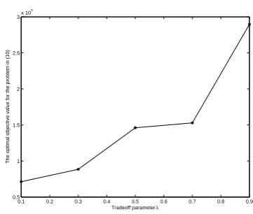
We considerλandαin (10) and (11) as parameters, and solve these problems for several values ofλandα. We first solve the problems for w1 = 1, w2 = 2, w3 = 3(instance
1), and then repeat the experiments forw1=w2=w3= 0
(instance 2). We obtain very similar results for both in-stances, hence we present results in Figures 1 and 2 only for instance 1. Note that after sampling the demands and the random amounts of cores that fall into each quality levels, the problems in (10) and (11) are formulated as two linear programming problems, which are then solved through CPLEX 12.2.
also be seen from the chance constraint in (6). Both Figures 1 and 2 reflect the increase in the conservatism of the system because the optimal objective value of the first-stage problem in (10) increases as λincreases in Figure 1, and it increases as αdecreases in Figure 2.
V. CONCLUSIONS AND FUTURE RESEARCH
In this paper, we consider a component, multi-product, periodic-review (re)assemble-to-order system, and find the joint optimal base-stock levels and component al-location policies in a risk-adjusted environment. We model this problem through a risk-adjusted two-stage stochastic programming problem, where the first-stage decisions are the base-stock levels for all components, and the second-stage decisions are the allocations of components to dif-ferent products. Risk adjustment is achieved through the conditional-value-at-risk constraint. We solve the resulting problem through the sample average approximation com-bined with the L-shaped method. Our preliminary numerical results are intuitively sound: as we make the system more conservative (by increasing the parameterλor by decreasing the parameterα), our expected total optimal objective value increases.
Further research should include more numerical results by using different multivariate distributions for demands. Con-sideration of market segmentation between remanufactured and manufactured products is a further important issue.
REFERENCES
[1] N. Agrawal and M. A. Cohen, “Optimal Material Control in an Assembly System with Component Commonality,” Naval Research
Logistics, vol. 48, pp. 409-429, 2001.
[2] Y. Akc¸ay and S. H. Xu, “Joint Inventory Replenishment and Component Allocation Optimization in an Assemble-to-order System,”Management
Science, vol. 50, no. 1, pp. 99-116, Jan. 2004.
[3] J. R. Birge and F. Louveaux,Introduction to Stochastic Programming, New York, USA: Springer-Verlag, 1997.
[4] F. Cheng, M. Ettl, G. Lin, and D. D. Yao, “Inventory-service Op-timization in Configure-to-order Systems,”Manufacturing & Service
Operations Management, vol. 4, no. 2, pp. 114-132, 2002.
[5] R. Geyer, L. Van Wassenhove, and A. Atasu, “The Economics of Remanufacturing under Limited Durability and Finite Product Life Cycles,”Management Science, vol. 53, no. 1, pp. 88-100, 2007. [6] V.D. R. Guide, V. Jayaraman, and J. D. Linton, “Building Contingency
Planning for Closed-loop Supply Chains with Product Recovery,”
Journal of Operations Management, vol. 21, pp. 259-279, 2003.
[7] G. Hadley and T. M. Whitin,Analysis of Inventory Systems, Englewood Cliffs, NJ, USA: Prentice Hall, 1963.
[8] W. H. Hausman, H. Lee, and A. X. Zhang, “Joint Demand Fulfillment Probability in a Multi-item Inventory System with Interdependent Order-up-to Policies,”European Journal on Operational Research, vol. 109, pp. 646-659, 1998.
[9] R. T. Rockafellar and S. P. Uryasev, “Optimization of Conditional Value-at-risk,”The Journal of Risk, vol. 2, pp. 21-41, 2000.
[10] A. Shapiro, D. Dentcheva, and A. Ruszczy´nski,Lectures on Stochastic
Programming: Modeling and Theory, Philadelphia, USA: SIAM, 2009.
0.1 0.2 0.3 0.4 0.5 0.6 0.7 0.8 0.9 0.5
1 1.5 2 2.5 3x 10
5
Tradeoff parameter λ
[image:5.595.334.515.141.294.2]The optimal objective value for the problem in (10)
Fig. 1. Effects of changingλon the optimal objective value of the first-stage problem in (10):α= 10%and fixed
0 0.02 0.04 0.06 0.08 0.1 0.12 0.14 0.16 0.18 0.2 0
2 4 6 8 10 12x 10
5
Significance level α
[image:5.595.335.515.510.663.2]The optimal objective value of the problem in (10)