Advance Access publication 2014 January 31
The relation between accretion rates and the initial mass function in
hydrodynamical simulations of star formation
Th. Maschberger,
1‹I. A. Bonnell,
2C. J. Clarke
3and E. Moraux
11UJF-Grenoble 1/CNRS-INSU, Institut de Plan´etologie et d’Astrophysique de Grenoble (IPAG) UMR 5274, F-38041 Grenoble, France
2Scottish Universities Physics Alliance (SUPA), School of Physics and Astronomy, University of St. Andrews, North Haugh, St. Andrews, Fife KY16 9SS, UK
3Institute of Astronomy, Madingley Road, Cambridge CB3 0HA, UK
Accepted 2013 December 11. Received 2013 December 11; in original form 2013 October 10
A B S T R A C T
We analyse a hydrodynamical simulation of star formation. Sink particles in the simulations which represent stars show episodic growth, which is presumably accretion from a core that can be regularly replenished in response to the fluctuating conditions in the local environment. The accretion rates follow ˙m∝m2/3, as expected from accretion in a gas-dominated potential, but
with substantial variations overlaid on this. The growth times follow an exponential distribution which is tapered at long times due to the finite length of the simulation. The initial collapse masses have an approximately lognormal distribution with already an onset of a power law at large masses. The sink particle mass function can be reproduced with a non-linear stochastic process, with fluctuating accretion rates∝m2/3, a distribution of seed masses and a distribution
of growth times. All three factors contribute equally to the form of the final sink mass function. We find that the upper power-law tail of the initial mass function is unrelated to Bondi–Hoyle accretion.
Key words: accretion, accretion discs – stars: formation – stars: luminosity function, mass function – open clusters and associations: general.
1 I N T R O D U C T I O N
The origin of the stellar initial mass function (IMF) is a key question for a theory of star formation. Several ideas have been proposed to explain the stellar IMF, for example fragmentation, competitive ac-cretion, a distribution of growth times, or, more statistically, space filling and gravoturbulent fragmentation. They succeed in explain-ing one or more properties of the IMF, such as its lognormal-like shape in the low-mass regime, the power-law behaviour at high masses (in particular the Salpeter exponent), its peak and its width. It is the purpose of this paper to investigate which of the ideas men-tioned above contribute to the development of the sink particle mass
functionin a hydrodynamical simulation of star formation(‘sink
particles’ are henceforth termed ‘sinks’ throughout the paper). We
aim in the process to shed some light on the origin of theobserved
IMF.
Fragmentation is one of the first processes proposed for star
formation, going back to Hoyle (1953) and extended by a
ran-dom component by Marcus (1968), Larson (1973), Elmegreen &
Mathieu (1983) and Zinnecker (1984). This random
fragmenta-tion, repeatedly splitting a fragment, is essentially a linear
stochas-tic process, first described by Kolmogorov (1941), that leads to a
lognormal distribution. The model of Marcus (1968)) predicts also
the total number of fragments in addition to their mass distribution.
E-mail:[email protected]
Another principal concept of star formation is stellar
accre-tion, either ˙m∝m2(Bondi–Hoyle) in stellar-dominated potentials
(Zinnecker 1982; Bonnell et al. 2001a,b) or ˙m∝m2/3 in
gas-dominated potentials (Bonnell et al.2001a,b). This leads to a
power-law behaviour of the mass function by spreading the initial seed distribution. In this model, the power-law exponent of the accretion rate–sink mass dependence is critical in determining the slope of
the upper power law of the IMF and Zinnecker (1982) used this
to relate the observed Salpeter exponent to Bondi–Hoyle accretion. In such models, the seed distribution is the random element, both the accretion rates and growth times are not assumed to have a distribution.
A third principal concept of star formation is the distribution of growth times. Accretion has to stop at some point, which is likely to be a random variable. Typically, an exponential distribution of
growth times is assumed (e.g. Myers2000,2009; Reipurth & Clarke
2001; Basu & Jones2004; Bate & Bonnell2005), which implies
that the probability for ‘killing’ growth is constant in time for each star. The distribution of growth times leads to a distribution in mass and affects the high-mass end of the mass function.
Gravoturbulent fragmentation, with its main theories of Padoan,
Nordlund & Jones (1997), Padoan & Nordlund (2002) and
Hennebelle & Chabrier (2008, 2009,2013) is based on counting
Jeans-unstable regions in a gas distribution that has lognormal den-sity fluctuations superimposed by turbulence. This is not so much related to the random splitting flavour of fragmentation mentioned
2014 The Authors
at University of St Andrews on September 9, 2014
http://mnras.oxfordjournals.org/
above, but more related to the process of random or subdivision of
a volume (Auluck & Kothari1954), which has also served in
sev-eral variations as explanation for the IMF (e.g. Auluck & Kothari
1965; Kiang1966; Richtler1994). The theories of gravoturbulent
fragmentation produce a mass function with a lognormal body and a power-law tail.
Several authors have attempted to combine one or more aspects,
for example: Basu & Jones (2004) combine a lognormal distribution
of seed masses with (deterministic) growth ˙m∝mor ˙m∝m2/3and
an exponential distribution of growth times. Bate & Bonnell (2005)
combine constant growth ( ˙m=const.) with a lognormal
distribu-tion of accredistribu-tion rates and an exponential distribudistribu-tion of growth times. [This is mathematically similar to random fragmentation models (apart from a change of sign of the quantity added); in the fragmentation models discussed above a uniform or Gaussian
in-stead of a lognormal distribution is typically used]. Myers (2011,
2012) investigates growth following ˙m=const.+m1.2with an
ex-ponential time distribution but without a distribution of seed masses.
Dib et al. (2010) consider deterministic growth ( ˙m∝m0.65) from a
seed mass distribution given by gravoturbulent fragmentation with
an exponential distribution of growth times. Maschberger (2013b)
discusses non-linear stochastic processes (a combination of random
fragmentation and accretion) with growth ˙m∝mαhaving a
lognor-mal distribution of accretion rates (due to the lognorlognor-mal distribution of turbulent density), with a distribution of seed masses and a dis-tribution of growth times. This is effectively a combination of all the processes discussed above, and we will use this prescription to model the sink mass function.
Numerical studies of star formation have been performed
on core scales (typically ≈1 M, 10 sinks; e.g. Goodwin,
Whitworth & Ward-Thompson2004a,b; Vorobyov & Basu2006,
2009; Krumholz, Klein & McKee 2007) on small cloud scales
(≈100 M, 100 sinks; e.g. Klessen2001; Bate, Bonnell & Bromm
2003; Schmeja & Klessen2004; Bate & Bonnell2005; Bate2009c,
2009b; Offner et al. 2009a, 2010; Commerc¸on, Hennebelle &
Henning 2011; Girichidis et al. 2011, 2012a,b; Hennebelle
et al. 2011; Seifried et al. 2011, 2012; Hansen et al. 2012;
Myers et al. 2013) and on star cluster scales (≈1000 M,
1000 sinks; e.g. Bonnell, Bate & Vine2003; Bonnell, Clark &
Bate 2008; Offner, Klein & McKee 2008; Bate 2009a, 2012;
Offner, Hansen & Krumholz 2009b; Peters et al. 2010a;
Bonnell et al.2011; Krumholz, Klein & McKee2011,2012).
Al-though the simulations employ different physical processes (isother-mal versus barotropic versus radiative transfer; wind feedback; mag-netic fields; etc.) they usually lead to a sink mass function fairly similar to the IMF, if enough sinks are formed.
There have been some comparisons of theoretical models with
simulations. For example, Schmidt et al. (2010) compare the core
distributions of their simulations with the models of Padoan &
Nordlund (2002) and Hennebelle & Chabrier (2008), while Bate
(2009a,2012) compares the sink mass function with the model of
Bate & Bonnell (2005). In this work, we set out to investigate the
simulation by Bonnell et al. (2008,2011) for the distribution and
mass dependence of the accretion rates, the distribution of growth times and the distribution of seed masses in order to find out what the parameters are and where, if there is any, the main random component of star formation originates.
This paper is structured as follows. In Section 2, we describe the calculation. An analysis of episodic growth and the classification of sink histories follow in Sections 3 and 4. The distribution and mass dependence of the accretion rates is analysed in Section 5. In Section 6, we discuss the location of each sink class in the mass
function and the distribution of initial collapse masses. Section 7 contains the analysis of the distribution of growth times. In Section 8, we investigate which one of the random elements, seed masses, accretion rates and growth times, is likely the main contributor to the shape of the IMF. A summary in Section 9 concludes the paper.
2 C A L C U L AT I O N
We analyse the calculation performed by Bonnell et al. (2008,2011),
to which we refer for further details. The initial cloud mass is
104M
, distributed over a cylinder 10 pc long and 3 pc in diameter.
There is a linear density gradient along the main axis, so at one end the cylinder is 33 per cent more dense than average and at the other end 33 per cent less dense. Turbulence is modelled by an initial divergence-free Gaussian random velocity field with a
power spectrum P(k) ∝ k4. Turbulence is not driven during the
calculation. At the start of the calculation the cloud is globally marginally unbound, but due to the density gradient bound in the upper half and unbound in the lower half.
Particle splitting (Kitsionas & Whitworth2002,2007) was used
to resolve fragmentation down to masses of 0.0167 M(equivalent
to 4.5 ×10⁷ smoothed particle hydrodynamics particles),
suffi-cient to resolve the formation of brown dwarfs. A lower resolution simulation was run initially to identify these regions in the initial conditions and the full simulation was then rerun, including the regions of higher resolution, in order to resolve the formation of all stars and brown dwarfs. The gas follows a barotropic equation of state,
P =kργ, (1)
where
γ =0.75; ρ≤ρ1
γ =1.0; ρ1≤ρ≤ρ2
γ =1.4; ρ2≤ρ≤ρ3
γ =1.0; ρ3≤ρ
(2)
and ρ1 = 5.5 × 10⁻¹⁹g cm−3, ρ2 = 5.5 × 10⁻¹⁵g cm−3 and
ρ3=2×10⁻¹³g cm−3. Star formation is modelled with sink
par-ticles (Bate, Bonnell & Price1995), which are created at a critical
density of 6.8×10⁻¹⁴g cm−3. The sink radius is 200 au and the
ac-cretion radius is 40 au, gravitational interactions are also smoothed at 40 au.
The simulation runs for about one free-fall time or 6.6×10⁵yr
and sinks start forming after≈1/2tff. In total 2542 sinks are formed
with masses ranging from 0.017 to 30 M. The vast majority of
the sink particles forms in the bound half of the cylinder and is concentrated in only a few rich subclusters.
This calculation has been first published by Bonnell et al. (2008)
who analysed it with respect to brown dwarf formation. The evolu-tion of subclusters, mass segregaevolu-tion on a subcluster scale and the upper end of the sink mass function (time variation of the exponent
and truncation) has been investigated by Maschberger et al. (2010).
Bonnell et al. (2011) discussed the star formation efficiency in
clus-tered and distributed regions. The properties of cores that form in
the simulation were analysed by Smith, Clark & Bonnell (2009a),
Smith, Longmore & Bonnell (2009b) and Smith et al. (2011),2012,
2013). Global mass segregation was covered in Maschberger &
Clarke (2011). Kruijssen et al. (2012) studied the dynamical
struc-ture of the subclusters, finding that they are close to virial equi-librium. The spatial and kinematic distribution of the sinks at the
at University of St Andrews on September 9, 2014
http://mnras.oxfordjournals.org/
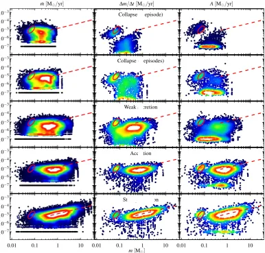
Figure 1. Examples of growth histories for each of the classes (C 1=collapse in 1 episode, C 2=collapse in 2 episodes, W A=weak accretion, A=accretion, S A=strong accretion). The left-hand plot shows the most massive sink in each class and the right-hand plot the first formed sink of each class. The left-hand panels show mass as a function of time, which is normalized in the middle panels (for comparison with Fig.5). The right-hand panels show the accretion rate as a function of time.
end of the calculation was dynamically evolved by Moeckel et al.
(2012), assuming instantaneous gas dispersal.
3 E P I S O D I C G R OW T H
Fig.1shows examples for the growth histories of some sinks
(sam-pling interval 1000 yr). The left-hand panels give mass as a function of time, which is also shown in the middle panels, but normalized to growth time and final mass (discussed in the next section). The right-hand panels show the accretion rate as a function of time. The alternating colour coding corresponds to the different episodes,
whose identification is discussed in the next section. Typicallym(t)
in the top rows has a concave shape which becomes gradually more
convex to the bottom row. Such a behaviour ofm(t) is also seen in
other simulations of star formation employing other codes and other
physical processes (see e.g. fig. 2 of Peters et al.2010b; fig. 12 of
Krumholz et al.2011; figs 14 and 15 of Girichidis et al.2012b; and
fig. 2 of Bonnell, Clarke & Bate2006).
The growth histories of the two top rows [i.e.m(t) and ˙m(t)] can
be understood as the collapse of an unstable core (cf. e.g. Foster &
Chevalier1993; Whitworth & Ward-Thompson2001), which leads
to a sharp rise of ˙m(t) followed by an exponential-like decay. Sink
particles are created during this collapse, instantaneously collecting all gas particles fulfilling the sink creation criteria, so that only part of the collapse is traced by the sink particle mass growth.
Particularly, if the increase of ˙m(t) is very fast the conditions for
sink formation are only satisfied when ˙m(t) is already decreasing
(top row of Fig.1). This behaviour of ˙m(t) is in agreement with the
properties of the bound cores (Smith et al.2011). ˙m(t) of these lower
mass sinks is comparable to Schmeja & Klessen (2004), Goodwin
et al. (2004a) or Girichidis et al. (2012b), which are starting with a
smaller gas mass.
In the lower panels, the sinks undergo several of these accre-tion/collapse episodes, which leads to sometimes severe variations
in ˙m, but lesser changes in the shape ofm(t). This is similar to the
fragmentation-induced starvation scenario of Peters et al. (2010a,b).
During each episode the accretion rate can be modelled by an ex-ponential increase or decrease as a function of time,
˙
m(t)=Aebt. (3)
A and bare different for each episode. This episodic growth is
reflected in the plot of the accretion rates as a function of mass.
Fig.2(top panel) shows ˙m(m) for the most massive sink of the
simulation (also shown in the bottom row of the left-hand plot in
Fig.1). Due to the episodic growth ˙mdoes not depend smoothly on
m, but shows ‘icicles’, where ˙mdrastically decreases andmis not
changing much. The simulations of Krumholz et al. (2012, fig. 13)
show a similar behaviour of ˙m(m).
●
● ● ●●●●●●●●●●●●●●●●●●●●●●●●●●●●●●●●●●●●●●●●●●●●●●●●●●●●●●●●●●● ● ● ● ● ●● ● ● ● ●● ● ● ● ●●●● ● ● ●●●●●●
●●● ●●●●●●●●●●●●●
● ●● ● ● ● ● ● ●● ●● ● ●●●●●●●●●●●
● ●● ●● ●●●●●
●●● ● ● ● ● ● ● ● ●●●●●●●
● ●● ● ● ● ● ● ● ● ● ● ●●●●● ● ● ● ● ● ● ● ● ● ● ● ● ● ● ●●●●●●●●●●●●●●●●●●●● ● ● ● ● ● ● ● ● ● ● ● ● ● ● ● ● ●●●●●●
● ● ● ● ●●●●●●
● ● ● ● ●●●●●● ●●●●● ● ●● ● ● ● ● ● ● ● ● ● ●
●
● ● ● ●●● ●● ● ●●●
●●●●●●●●●●●●●●●●●●●●
●●●●●●●●
●●● ●●
● ●●●●●●●●●●●
●●●● ● ● ● ● ●● ●
● ● ●● ● ● ● ●●●● ● ● ●●●●●●
● ●●●●●●
● ●●●●●●
● ● ● ●
● ● ● ● ● ● ●● ●● ●●●●●●●●●●●●●●●
●●
●●●● ● ● ● ● ● ●
● ● ● ● ● ●●● ● ●●● ● ●● ● ● ●
● ● ● ● ●
● ●●●● ●
● ● ● ● ● ● ● ● ● ● ● ● ● ●●●●●●●●●●● ● ● ● ● ● ● ●
● ● ● ● ● ● ● ● ● ● ●
● ● ● ● ● ● ● ● ● ● ● ● ● ●
● ● ● ● ●●●●●●
● ● ● ● ● ● ● ●
● ● ● ● ● ● ● ● ● ● ● ● ● ● ● ● ●
● ●
●
● ●
●
● ●● ●●
● ● ●●●●●●
● ● ● ●●●●●
● ●
● ● ● ● ● ● ● ●●●●●
Figure 2. Top panel: accretion rate as a function of mass for the most massive sink particle. Episodes have been colour coded alternatingly. Bottom panel: absolute value of the fitted exponentαof the accretion rate ˙m∝mα for each episode. The arrows show the sign ofα, downwards for negativeα and upwards for positiveα. Note the logarithmic axis for the exponent.
at University of St Andrews on September 9, 2014
http://mnras.oxfordjournals.org/
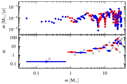
[image:3.595.317.535.532.676.2]The lower panel of Fig.2shows the absolute values for exponent
of a fit ˙m∝mα in each episode on a logarithmic scale. Upwards
arrows indicate a positive exponent (increasing ˙m) and downwards
arrows a negative exponent (decreasing ˙m). There are large
varia-tions inα. Although there are some episodes withα≈2, generally
we obtain much larger values during an episode. It is thus hard to explain the form of the sink mass function in terms of the Bondi–
Hoyle accretion model proposed by Zinnecker (1982).
The episodic accretion that is described here is due to the re-peated creation and depletion of a gas core around a sink particle
while the star gains most of its mass. This is different from the episodic accretion described in Stamatellos, Whitworth & Hubber
(2011,2012) which operates in discs smaller than the sink radius of
our calculation located in cores that are not replenished. Also, the episodic accretion here has to be distinguished from bursty accre-tion during a T Tauri or FU Orionis phase occurring only after most
of a star’s mass has been assembled (cf. Vorobyov & Basu2006,
2009).
4 C L A S S I F I C AT I O N O F T H E S I N K S
4.1 Identification of the episodes
We determine the episodes from behaviour of the rolling mean accretion rate as a function of time,
˙
m(ti+5)= 1 11
i+11
k=i
˙
m(tk). (4)
The time window used is 11 000 yr, or 11 data points, which we found to be a reasonable compromise between the smoothness of the mean accretion rate and the resolution of the episodes. The beginning and end of an episode is characterized by a sign change
in the numerical derivative of ˙m(ti). We calculate the sign at timeti
from five data points with
sign(ti)=m˙(ti−2)−m˙(ti+2). (5)
If the sign changes fromtitoti+1then a new episode starts atti+1.
This procedure leads to some very short episodes, which typically last only a few thousand years. These are only spurious detections. Therefore, we remove them (pruning) by attaching any episode that is shorter than 5000 yr (less than five data points) to the previous
episode. The colour coding in Figs1and 2shows the episodes
identified in this way. Our episode determination finds the main features in the growth history roughly agreeing with what would be found by human eye.
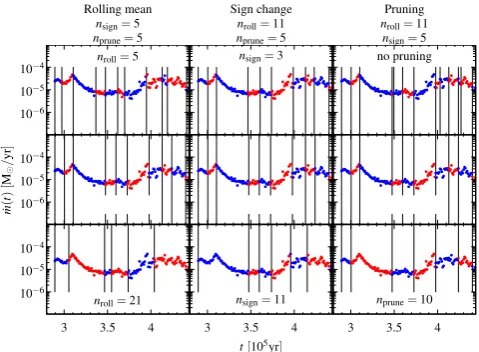
Fig.3shows the effects of parameter variations in the episode
determination algorithm using the first formed strongly accreting sink as an example. For clarity, only a part of the growth history
is shown (complete in the bottom-right panels of Fig.1). The
ver-tical lines show the boundaries of the episodes for the parameter choice of the respective panel. There are three parameters in the episode detection algorithm, the number of data points over which
the rolling mean runs (nroll), the number of data points over which
the sign change is determined (nsign) and the maximum length of
episodes which are pruned (nprune). In each column of Fig.3one
of the parameters is varied (the used value is given in the panel), whereas for the other parameters our standard choice is used (given on top of the panel). The panels in the middle row are identical, corresponding to our adopted choice of parameters, and are shown for easier comparison. For this particular sink, the algorithm should
find the first three episodes which are a decreasing ˙mfrom initial
●●●●●●●●●●●●●●●●●●●●●●●●●●●●●●●●●●●●●●●●●●●●●●●●●●●●●●●●●●●●●●●●●●●●●●●●●●●●●●●●●●●●●●●● ● ●●●●●●●●●●●●●●●
●●● ●●●●●●●●●●●●●●●●●●●●●●●●●●●●●●●●●●●●●●●●●●●●●
● ●●●●●●
●●●●●●●●●●●●●●●●●●●●●●● ●●●●●
●●●●●●● ●●●●●●●●●●
●●●●●●●●●●●●●●●●●●●●●●●●●●●●●●●● ●●●●●●●●●
●●●●●●●● ●●● ● ●●●●●●
●
●● ● ● ●●●●
●●● ●● ●●●●●●●●●●●●●●●●●●●●●●●●●●●●
●●●●●
●●●●●
●●●●●●●●●●●●●●●●●●●●●●●●●●●●●●●●●●●●●●●●●●●●●●●●●●●●●●●●●●●●●●●●●●●●●●●●●●●●●●●●●●●●●● ●●●●●●●●●●●
● ●●●●●●
●●● ●●●●●●●●●●●●●●●●●●●●●●●●●●●●●●●●●●●●●●●●●●●●●●●●●●●● ●●●●●●●●●●●●●●●●●●●●●●●
●●●●●●●●●●●● ●●●●●●●●●●●●●●●●●●●●●●●●●●●●●●●●●●●●●●●●●●
●●●●●●●●●●● ●●●●●●
●●● ● ●●●●●●
●●● ●
● ●●●●
●●● ●● ●●●●●●●●●●●●●●●●●
●●●●●●●●●●●●●●●
●●●● ●●
●●●●●●●●●●●●●●●●●●●●●●●●●●●●●●●●●●●●●●●●●●●●●●●●●●●●●●●●●●●●●●●●●●●●●●●●●●●●●●●●●●●●●●●●●●●●●●●●●●●●●●●● ●●●
●●●●●●●●●●●●●●●●●●●●●●●●●●●●●●●●●●●●●●●●●●●●●●●●●●●●
●●●●●●●●●●●●●●●●●●●●●●●●●●●● ●●●●●●●●●●●●●●●●●
●●●●●●●●●●●●● ●●●●●●●●●●●●●●●●●●●
●●●●●●●●●●●●●●●●● ●●● ● ●●●●●●
●●● ● ● ●●●●
●
●● ●● ●●●●●●●●●
●●●●●●●●●●●●●●●●●●● ●●●●●
●●●●●
●
●●●●●●●●●●●●●●●●●●●●●●●●●●●●●●●●●●●●●●●●●●●●●●●●●●●●●●●●●●●●●●●●●●●●●●●●●●●●●●●●●●●●●●● ●●●●●●●●●
● ●●●●●●
●●● ● ●●●●●●●●●●●●●●●●●●●●●●●●●●●●●●●●●●●●●●●●●●●●
●●●●●●● ●●●●●●●●●●●●●●●●●●●●●●●
●●●●● ●●●●●●●
●●●●●●●●●●●●●●●●●●●●●●● ●●●●●●●●●●●●●●●
● ●●●
● ●●●●●●●●
● ● ●●●●●●
●●● ● ● ●●●●●
●●● ● ●
● ●●●●●●
●● ●●●●●●●●●●●●●●●●●●●●●●●●●●●●
●●●●● ●●●●●
●
●●●●●●●●●●●●●●●●●●●●●●●●●●●●●●●●●●●●●●●●●●●●●●●●●●●●●●●●●●●●●●●●●●●●●●●●●●●●●●●●●●●●● ●●●●●●●●●●●
● ●●●●●●
●●● ● ●●●●●●●●●●●●●●●●●●●●●●●●●●●●●●●●●●●●●●●●●●●●●●●●●●● ●●●●●●●●●●●●●●●●●●●●●●●
●●●●●●●●●●●● ●●●●●●●●●●●●●●●●●●●●●●●●●●●●●●●●●●●●●●●●●●
● ●●●●●●●●●●
●●●●●● ●●● ● ● ●●●●●
●●● ●
● ● ●●●●●●
●● ●●●●●●●●●●●●●●●●●
●●●●●●●●●●●●●●●
● ●●● ●●
●
●●●●●●●●●●●●●●●●●●●●●●●●●●●●●●●●●●●●●●●●●●●●●●●●●●●●●●●●●●●●●●●●●●●●●●●●●●●●●●●●●●●●●●●●●●●●●●●●●●●●●●● ●●● ● ●●●●●●●●●●●●●●●●●●●●●●●●●●●●●●●●●●●●●●●●●●●●●●●●●●●
●●●●●●●●●●●●●●●●●●●●●●●●●●●● ●●●●●●●●●●●●●●●●●
●●●●●●●●●●●●●●●●●●●●●●●●●●●●●●●● ● ●●●●●●●●
● ● ●●●●●●
●●● ● ● ●●●●●
●●● ● ● ● ●●●●●●
●● ●●●●●●●●●
●●●●●●●●●●●●●●●●●●● ●●●●●
●●●●●
●●●●●●●●●●●●●●●●●●●●●●●●●●●●●●●●●●●●●●●●●●●●●●●●●●●●●●●●●●●●●●●●●●●●●●●●●●●●●●●●●●●●●●●● ●●●●●●●●●
● ● ●●●●●●●●●●●●●●●●●●●●●●●●●●●●●●●●●●●●●●●●●●●●●●●●●●●●●
●●●●●●● ●●●●●●●●●●●●●●●●●●●●●●●
●●●●● ●●●●●●●
●●●●●●●●●● ● ●●●●●●●●●●●●●●●●●●●●●●●●●●●●
●●● ● ●●●●●●●●
●●●●●●●● ●●●
● ●●●●●●
●●● ●●●●●●
●●● ●● ●●●●●●●●●●●●●●●●●
●●●●●●●●●●● ●●●●● ●●●●●
●●●●●●●●●●●●●●●●●●●●●●●●●●●●●●●●●●●●●●●●●●●●●●●●●●●●●●●●●●●●●●●●●●●●●●●●●●●●●●●●●●●●●● ● ●●●●●●●●●●●●●●●●●
● ●● ● ●●●●●●●●●●●●●●●●●●●●●●●●●●●●●●●●●●●●●●●●●●●●●●●●●●● ●●●●●●●●●●●●●●●●●●●●●●●
●●●●●●●●●●●● ●●●●●●●●●●
● ●●●●●●●●●●●●●●●●●●●●●●●●●●●●●●●
● ●●●●●●●●●●
● ●●●●●●●●
● ●●●●●●
●●● ●●●●●●
●●● ●● ●●●●●●●●●●●●●●●●●
●●●●●●●●●●●●●●●
●●●● ●●
●●●●●●●●●●●●●●●●●●●●●●●●●●●●●●●●●●●●●●●●●●●●●●●●●●●●●●●●●●●●●●●●●●●●●●●●●●●●●●●●●●●●●●●●●●●●●●●●●●●●●●●● ● ●● ● ●●●●●●●●●●●●●●●●●●●●●●●●●●●●●●●●●●●●●●●●●●●●●●●●●●●
●●●●●●●●●●●●●●●●●●●●●●● ●●●●●
●●●●●●●●●●●●●●●●● ● ●●●●●●●●●●●●●●●●●●●●●●●●●●●●●●●
● ●●●●●●●●
●●● ●●●●●●●●
● ●●●●●●
●●● ●●●●●●
●●● ●● ●●●●●●●●●
[image:4.595.309.549.56.232.2]●●●●●●●●●●●●●●●●●●● ●●●●● ●●●●●
Figure 3. Effects of the parameter choice on the episode detection. The middle row shows the same plot three times for easier comparison.
collapse (2.9–3×10⁵yr) and then rise (3–3.1×10⁵yr) and again
decrease (3.1–3.5×10⁵yr) of ˙mof the first accretion event. Up
to approximately 3.7×10⁵yr the accretion rate is rather smooth
during the episodes, but afterwards there is a larger amount of fluc-tuation, which makes episode detection more difficult.
Averaging over a shorter period produces more episodes (top-left panel), whereas a longer averaging period produces less episodes
(bottom-left panel). Changingnsign has the same effect. Without
pruning many very short episodes are produced (after 4×10⁵yr,
top-right panel), but if the pruning length is very long then real episodes are lost (bottom-right panel). Generally, larger values of the parameters give longer episodes but miss some short ones, while smaller parameter values lead to shorter episodes but more spurious detections. Our choice of parameters is a compromise between the number and length of episodes.
4.2 Classification of the growth histories
The growth history of a sink consists of a collapse phase often followed by an accretion phase, consisting of one or many episodes. The collapse phase falls normally into a single episode, but can sometimes extend over two episodes, About half of the sinks show significant growth by accretion after the initial collapse phase. Most sinks show a quiescent phase of very minor mass gain that occurs in the later stages of their evolution, after the initial collapse and any subsequent accretion phases. Mass growth has effectively stopped when they set in. Therefore, we define the growth time of a sink (t95 per cent) as the time during which 95 per cent of the final mass is
assembled. The parts of the growth histories that fall aftert95 per cent
are shown in black in Fig.1. Typically, the time betweent95 per cent
and the end of the simulation covers the final quiescent phase, except for massive sinks, where some accretion is needed for the last 5 per cent of mass gain. Quiescent phases can also occur between
two accretion events beforet95 per cent.
This leads us to the following classification scheme for the growth histories of the sinks.
(0)Unresolved collapse. Sinks that less than double their initial mass during the simulation.
(ia)Collapse in 1 episode. Sinks that have 75 per cent of their
mass gain (mend−mstart) in the first episode and are not class (0).
at University of St Andrews on September 9, 2014
http://mnras.oxfordjournals.org/
(ib)Collapse in 2 episodes. Sinks that have 75 per cent of their mass gain within the first two episodes and are not class (0) or (ia). (ii)Weak accretion. Sinks that achieve at least 50 per cent of their final mass in less than the first 33 per cent of their growth time (t95 per cent) and are not class (0), (ia) or (ib).
(iii)Accretion. Sinks that achieve at least 50 per cent of their final
mass in the time between 33 and 50 per cent of their growth time and are not class (0), (ia) or (ib).
(iv)Strong accretion. Sinks that achieve more than 50 per cent of their final mass in the second half of their growth time and are not class (0), (ia) or (ib).
For the classification, we first establish whether a sink falls into class (0) or not. If the sink more than doubles the mass, it con-tains enough data points to proceed with the analysis and clas-sification. The next step is to establish whether a sink that dou-bles in mass is collapsing [class (ia) or (ib)] or not. If the mass gain of a sink is not dominated by the initial collapse then signif-icant amounts of accretion are present and it can be classified as weakly/intermediate/strongly accreting (classes (ii), (iii) or (iv)). The condition for being in class (ii), (iii) or (iv) is mutually exclu-sive. Thus, the classification of a sink is unique, it is assigned only one class. Note that the classification scheme is independent of the final sink mass and only based on the morphology of the growth history.
Sinks in class (0) have more than half of their final mass already at the moment when the sink is formed during the first collapse phase. Therefore, they are collapse dominated, but their growth history is not resolved by the sink particle, only by the gas particles. Usually they have very small masses.
The typical behaviour of each class is schematically represented
[image:5.595.318.534.51.478.2]in Fig.4, which has the same layout as Fig.1. The left-hand panels
Figure 4. Schema of episodic growth for each class. The left-hand panels showm(t), which has been normalized in the middle panels. The right-hand panels show ˙m(t). For class (ia) in the top panel the dotted red curve shows the initial episode, which is not resolved in the simulation. The black bar in panels (ii), (iii) and (iv) runs from1
3t95 per centto
1
2t95 per centat half the final
[image:5.595.43.284.420.666.2]sink mass.
Figure 5. Characteristic growth histories of the sinks for each class, which change with increasing amount of accretion from a concave shape to a convex shape. Time is normalized ast/t95 per centand mass is normalized to the final mass of the sink.
showm(t), the middle panels the normalizedm(t) and the right-hand
panels ˙m(t). Fig.5shows the characteristic growth histories for all
sinks in each of the classes (normalized mass versus normalized
time, corresponding to the middle panels of Figs1and 4). This
allows us to show all sinks despite their differing masses and growth times in order to see the variations of the growth histories in each class. The dots are the growth histories of each sink, colour coded to the point density at their location.
Sinks of class (ia) and (ib) are collapsing cores that do not undergo any significant further accretion. The signature of a collapse in the
˙
m−tplot is a very sharp rise of ˙mfollowed by a more gentle decline.
As the increase of ˙mcan be very fast it is not always completely
traced by a sink particle, sometimes the sink is formed only when ˙m
is already declining. Then most of the mass is gained in the single
episode of declining ˙m. This is the case for sinks of class (ia), shown
in the top panels of Figs1,4and5. In Fig.5, the bulk of the sinks
behaves as in the schema, but at small values of the normalized time another branch appears in the upper part. The top branch is due to
at University of St Andrews on September 9, 2014
http://mnras.oxfordjournals.org/
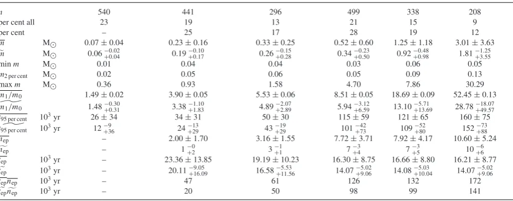
Table 1. Properties of each category. Bars denote average values which are quoted with the standard deviation. Tildes denote the median with the errors corresponding to the quantiles at±1σ(83 and 17 per cent). The rows are:nnumber of sinks in this class; ‘per cent all’ is the percentage with respect to all sinks; per cent is with respect only to the mass gaining sinks;mis final mass; minmis the minimum mass of a class, which is affected by outliers. Therefore, we give also the 2 per cent quantile (m2 per cent); maxmis the maximum mass of a class;m1/m0is mass gain (ratio final/initial mass);t95 per centis growth time;
nepis number of episodes; andtepis duration of episodes.
(0) Unresolved collapse (ia) Collapse (1 episode) (ib) Collapse (2 episodes) (ii) Weak accretion (iii) Accretion (iv) Strong accretion
n 540 441 296 499 338 208
per cent all 23 19 13 21 15 9
per cent – 25 17 28 19 12
m M 0.07±0.04 0.23±0.16 0.33±0.25 0.52±0.60 1.25±1.18 3.01±3.63
m M 0.06+−00..0204 0.19−+00..1710 0.26−+00..1528 0.34−+00..2350 0.92−
0.48
+0.98 1.81−+13..2555
minm M 0.01 0.04 0.04 0.03 0.06 0.05
m2 per cent M 0.02 0.05 0.06 0.05 0.09 0.13
maxm M 0.36 0.93 1.58 4.70 7.86 30.29
m1/m0 1.49±0.02 3.90±0.05 5.53±0.06 8.51±0.05 18.69±0.09 52.45±0.13
m1/m0 1.48−+00..3031 3.38−
1.10
+1.83 4.89−
2.07
+2.89 5.94−
3.12
+6.59 13.10−
5.71
+13.69 28.78−
18.07
+49.57
t95 per cent 103yr 26±34 34±31 50±30 115±59 121±65 160±75
t95 per cent 103yr 12−+936 24−
13
+29 43− 19
+29 101− 42
+73 109− 52
+80 152− 73
+88
nep – 2.00±1.70 3.16±1.55 7.72±3.71 7.92±4.17 10.60±5.24
nep – 1−+02 3+−11 7−+34 7−+35 10−
6
+6
tep 103yr – 23.36±13.85 19.19±10.23 16.30±8.75 16.66±8.80 16.21±8.77
tep 103yr – 20.11+−169.05.09 16.58−
5.53
+11.56 14.07−
5.02
+9.06 14.08−
5.03
+10.04 14.07−
5.02
+9.06
tepnep 103yr – 47 61 126 132 172
tepnep 103yr – 20 50 98 99 141
(very low mass) sinks that gain a very large fraction of their mass in the collapse, but do not quite reach 95 per cent of their final mass. A small accretion event is needed to reach the final mass, which can occur a rather long time after the collapse. An example for this is the first sink formed of class (ia), shown in the top-right part of Fig.1.
Sinks in class (ib) are formed very early on during the initial
collapse and the quickly rising ˙mis resolved, so that two episodes
are found. Their behaviour is shown in the second panels from top
in Figs1,4and5. Compared to class (ia) the scatter has increased
in Fig.5and the top branch is not present any more. Class (ia) can
by construction only contain collapsing sinks, whereas class (ib) can contain sinks that had an accretion episode after collapse, if the
initial rise of ˙mis unresolved. We did not find a robust and objective
way to distinguish between 2-episode collapse and 1-episode plus an accretion episode in class (ib). Therefore, we introduced the split of collapsing sinks into classes (ia) and (ib).
Classes (ii), (iii) and (iv) contain sinks that underwent increasing magnitudes of accretion and have more episodes than the sinks in classes (ia) and (ib). Accretion does not proceed in a smooth way, perhaps with some scatter in the accretion rates, but as a sequence of accretion events after the initial collapse. This is particularly visible
in the bottom panels for ˙m(t) of Fig.1which has a zigzag shape
from the sharp rise and decline of ˙mduring the secondary ‘accretion
collapses’. However, our classification scheme is for those sinks not
based on the ˙m(t), but on the time when the majority of mass is
acquired. The lower three panels of Fig.4for accreting sinks show
a black bar which runs from 13t95 per centto 12t95 per centat half of the
final mass.m(t) for the weakly accreting sinks [class (ii)] runs to the
left of the bar, for accreting sinks [class (iii)] it goes through the bar,
and strongly accreting sinks [class (iv)] havem(t) that goes below
the bar. The change ofm(t) from convex [class (ii)] via linear [class
(iii)] to concave [class (iv)] is easier to identify than the change in
behaviour of ˙m(t) (see Fig.1). In the lower three panels of Fig.5
this change of morphology is well visible.
4.3 Properties of the sink classes
Table1gives some characteristic quantities for each sink class where
bars denote the mean and tildes the median. As the distributions of these quantities are very skewed the standard deviation can be larger than the average. Therefore, we also give with the median mass
the quantiles corresponding to±1σ (83 and 17 per cent). About
23 per cent of all sinks do not double their mass during their stay in the simulation. Of those that significantly gain mass 40 per cent
only collapse (classes ia and ib),≈30 per cent show weak accretion
(ii),≈ 20 per cent are accretion dominated (iii) and≈10 per cent
have strong accretion (iv). There is a steady increase in the mean and median mass of each class (but note that mass is not a criterion for classification). The minimum mass in each class is probably affected by some outliers due to misclassification, hence we also provide the 2 per cent quantile. Collapsing sinks have on average
a mass of≈0.3 M, but strongly accreting sinks are a factor of
10 more massive. Similarly, the average mass gain (ratio of final
and initial mass,m1/m0) ranges from a factor of≈4 up to a factor
of≈50. With increasing amount of accretion also the growth time
increases, as well as the number of episodes (nep). The duration of
the episodes (tep), however, is fairly constant for each class and not
much affected by the presence and amount of accretion.
5 AC C R E T I O N R AT E S
5.1 Mass dependence of the accretion rates
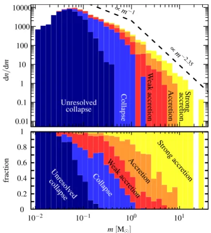
Fig.6shows the accretion rate as a function of mass for all sinks in
the simulation at all sampling times. The dots are colour coded to the point density at their location. Accretion events can be discrete because of the discrete modelling of the gas density so that there appear stripes of points at the bottom of the plot. This corresponds to the accretion of a one single, two, etc. gas particles to the sink during the sampling time interval. Sampling intervals without any
at University of St Andrews on September 9, 2014
http://mnras.oxfordjournals.org/
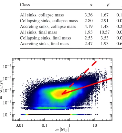
Table 2. Results from the mass function fits.α,βandμare the parameters of theL3IMF.αis the high-mass exponent andγthe low-mass exponent.mγandmαare the masses below or above which theL3IMF follows power laws. The mode refers to the maximum ofL3in linear units (as Fig.10), whereasmPeakrefers to the maximum in logarithmic units.
Class α β μ γ mγ mα Mode mPeak Average mass
All sinks, collapse mass 3.36 1.67 0.18 −0.58 0.078 0.42 0.09 0.15 0.19 Collapsing sinks, collapse mass 2.80 2.91 0.07 −2.44 0.021 0.20 0.06 0.09 0.15 Accreting sinks, collapse mass 4.19 1.48 0.28 −0.52 0.150 0.53 0.15 0.22 0.23 All sinks, final mass 1.93 10.57 0.01 −7.90 0.002 0.11 0.06 0.15 0.67 Collapsing sinks, final mass 2.53 3.53 0.05 −2.88 0.015 0.20 0.06 0.10 0.19 Accreting sinks, final mass 2.47 1.93 0.67 −0.37 0.173 2.60 0.18 0.64 1.25
Figure 6. Plot of the accretion rates versus m for all sinks at all times of the simulation, colour coded to the point density. Lines are for ˙m∝m2(dashed)
and ˙m∝m2/3(solid). Time intervals with no accretion have been assigned
a fiducial accretion rate of 10−7M
yr−1.
accretion of a gas particle, which are not uncommon, are shown as
the stripe at 10−7M
yr−1.
Below≈0.5 Mthe accretion rates appear to be independent of
the sink mass, although there is a slight trend of a decrease of ˙m
withm. Above≈0.5 Mthe accretion rates increase with mass,
following approximately ˙m∝m2/3. This is predicted for accretion
in gas-dominated potentials (Bonnell et al.2001a,b). Certainly the
sinks do not follow classical Bondi–Hoyle accretion∝m2, which
corresponds to the dashed line. Besides the mass scaling there is a considerable scatter in the accretion rates, spanning more than an order of magnitude. Furthermore, there are the ‘icicles’ in the
˙
m–mplot, strands of decreasing accretion rates at the same mass,
which belong to the same sink. These are particularly visible at large masses.
The mass dependence of the accretion rates has been studied by
several authors. For small masses (m <0.5 M) Bate & Bonnell
(2005), Bate (2009a,c,2012) find no mass dependence of the
time-averagedm˙, which is consistent with Fig.6. Offner et al. (2009a)
fit also thetime-averagedaccretion rates and find ˙m∝m0.64
with-out radiative transfer and ˙m∝m0.92including radiative transfer in
the calculation. Dib et al. (2010) report that in the simulations of
Schmeja & Klessen (2004) thefinalmasses scale with the peak
accretion rate as ˙mpeak∝m0final.65. However, as very likely in these
simulations sink growth is episodic as in ours, the time-averaged or peak accretion rate may not necessarily give the appropriate mass scaling.
5.2 Accretion rates of the individual classes
With the grouping of the sinks in various growth classes we are
able to disentangle Fig.6. This is done in Fig.7, which shows ˙m
versusmfor each class individually. The left-hand column gives
˙
m–m sampled at 1000 yr intervals where the ‘icicles’ of
expo-nentially decaying accretion rates are well visible. Again we add
10−7Myr−1 to the accretion rate in order to be able to show
episodes of extremely low or no accretion in the logarithmic plot.
As the episodic accretion produces a large spread in ˙mwe show
in the middle column of Fig. 7the average accretion rates
dur-ing each episode. This is given by the fraction of mass accreted
during an episode, m, divided by the duration of the episode,
t. The mass coordinate is the mass at the beginning of the
episode. Here many of the ‘icicles’ have vanished and the scatter is
reduced. The average accretion ratesm/tduring an episode
de-pend on the length of the episode. In order to assess the length
dependence we show in the right-hand panel of Fig.7the scaling
constantAof a fit ˙m=Aebt as a function ofmat the beginning of
an episode.Ashows the same behaviour as ˙m−morm/t−m,
in particular the samem2/3scaling. Compared tom/t−mthere
is more scatter in the distribution ofA.
In the middle and left-hand column of Fig.7, it is very evident
that there are three types of episodes: initial collapse, accretion
and quiescent. The initial collapse is located at ≈0.08 M and
10−5M
yr−1, marked by an ellipse. This phase is well separated
from the two others. For the strongly collapsing sinks in one phase the initial collapse is followed mainly by quiescent phases, although some subsequent accretion occurs on a small level. The quiescent
phases are located below 10−6M
yr−1at the bottom of the panels.
Accretion is at a higher ˙m, steadily increasing from panel to panel
downwards. Finally, for the accreting or strongly accreting sinks (class iii/iv) a very clear mass dependence of the accretion rates
becomes evident, scaling∝m2/3(dashed line). This scaling is
ex-pected from accretion in a gas-dominated potential (Bonnell et al.
2001a,b). As accretion increases quiescent phases become more and more rare.
The instantaneous accretion rates in the left-hand column of Fig.7
show similar trends as the in middle and right-hand column. How-ever, due to the exponential time dependence of the accretion rates the features are smeared out, particularly the collapse phase. Also, this leads to a very strong population of very small accretion rates.
5.3 Fluctuations in the accretion rates
The time-averaged accretion rates show besides their mass depen-dence a large scatter, which can be written as
m
t =m
2/3W,
(6)
whereWis a fluctuating quantity generating the scatter in the
ac-cretion rates. In order to estimate the amount of scatter, we need to
determine the distribution ofWwith its parameters. The strongly
accreting sinks have the widest mass range over which they
fol-low ˙m∝m2/3. Therefore, we analyse the distribution ofWfor the
at University of St Andrews on September 9, 2014
http://mnras.oxfordjournals.org/
[image:7.595.66.279.93.324.2]Figure 7. Left-hand panel: accretion rates as a function of sink mass for each class. Middle panel: episodic accretion rate, defined as mass gain during an episode,m, per duration of episode,t, as function of the sink mass at the beginning of the episode. Right-hand panel: scaling constantAof a fit ˙m=Aebt for each episode versus the sink mass at the beginning of the episode. Three groups of episodes become visible, a collapse type (red ellipse), an accreting type where ˙m∝m2/3(dashed line) and quiescent episodes below≈10−6M
yr.
strongly accreting sinks, shown in Fig.8. The top panel showsWas
a function of the sink mass. Like in Fig.7the three types of episodes
are visible, collapsing, quiescent and accreting. As the mass
depen-dence forWis removed, the distribution ofWis constant in mass.
It appears that during accreting episodes (marked in red)Wfollows
a lognormal distribution,
p(W)= 1
W
1
√
2πσWe
−1 2
(logW−μW)2
σ2
W . (7)
Accreting episodes are selected by requiring that W >
10−6 M1/3
yr−1 and m >0.5 M
(shown as red dots). A
maxi-mum likelihood fit of the parameters of a lognormal distribution
givesμW= −11.44 andσW=0.74.
In order to test the goodness of a lognormal fit we show in the
bottom panel of Fig.8a histogram ofW, selecting all those with
m >0.5 M(including quiescent episodes). The red shaded his-togram shows a lognormal distribution with the estimated
parame-ters. Above 10−6M1/3
yr−1the distribution ofWagrees reasonably
with the lognormal fit, but below 10−6M1/3
yr−1there is an excess
of smallW. The low-Wpart of the distribution contains mainly
quiescent episodes, and is thus not representative for the
distribu-tion ofWduring accreting episodes. Therefore, the assumption of a
lognormal distribution ofWduring accreting episodes is justified
by the data.
6 L O C AT I O N O F T H E C L A S S E S I N T H E S I N K M A S S F U N C T I O N A N D D I S T R I B U T I O N O F I N I T I A L C O L L A P S E M A S S E S
Our classification of the growth histories is independent of the final mass and the growth time of each sink. It merely depends on the behaviour and shape of the growth history. Within the framework
of gas-dominated competitive accretion (Bonnell et al.2001a,b). it
is expected that massive stars gain most of their mass via accre-tion of initially unbound gas after the collapse of the initial core. As our classification groups the sinks according to the amount of post-collapse accretion that they undergo, we would expect that the strongly collapsing sinks without much accretion populate the low-mass range, whereas the strongly accreting sinks have large
masses. This is exactly what we find. Fig.9shows in the top panel
a histogram of the final sink masses divided into the classes. The amount of accretion in a sink’s growth history increases with in-creasing final sink mass. The overall shape of the final sink mass function has three main components, a lognormal-like low-mass
at University of St Andrews on September 9, 2014
http://mnras.oxfordjournals.org/