1 2 3 4 5 6
Line Transect Sampling of Primates: Can Animal-to-Observer
Distance Methods Work?
Stephen T. Buckland • Andrew J. Plumptre • Len Thomas • Eric A. Rexstad
S. T. Buckland([email protected]) 7
8 9 10 11 12 13 14 15 16 17 18
S. T. Buckland • L. Thomas • E. A. Rexstad
Centre for Research into Ecological and Environmental Modelling, University of St Andrews, The Observatory, Buchanan Gardens, St Andrews, Fife KY16 9LZ, UK
A. J. Plumptre
Wildlife Conservation Society, PO Box 7487, Kampala, Uganda
Short title: Use of AODs in line transect sampling
19 20 21 22 23 24 25 26 27 28 29 30 31 32 33 34 35 36 37 38 39 40 41 42 43
Line Transect Sampling of Primates: Can Animal-to-Observer
Distance Methods Work?
Stephen T. Buckland • Andrew J. Plumptre • Len Thomas • Eric A. Rexstad
Abstract Line transect sampling is widely used for estimating abundance of primate populations. Animal-to-observer distances (AODs) are commonly used in analysis, in preference to perpendicular distances from the line. This is in marked contrast with standard practice for other applications of line transect sampling. We formalize the mathematical shortcomings of approaches based on AODs, and show that they are likely to give strongly biased estimates of density. We review papers that claim good performance for the method, and explore this performance through simulations. These confirm strong bias in estimates of density using AODs. We conclude that AOD methods are conceptually flawed, and that they cannot in general provide valid estimates of density.
Keywords animal-to-observer distances • distance sampling • estimating primate density • Kelker strip • modified Kelker method • primate surveys
Introduction
44 45 46 47 48 49 50 51 52 53 54 55 56 57 58 59 60 61 62 63 64 65 66 67 68 69
Distance (Thomas et al., in press). However, methods that in other disciplines are generally considered to be obsolete are still often used and recommended in primatology: the Kelker strip (Kelker, 1945) and the ‘modified Kelker method’ (Struhsaker, 1981), which covers a range of methods based on assessing the effective width of the searched strip from animal-to-observer distances or AODs. In addition, survey design issues are often ignored, and the precision of abundance estimates is often not quantified, compromising studies designed to compare the performance of different methods.
In this paper, we first consider strip transect sampling, and the assumptions under which it is effective. We then explore AOD methods that are conceptually related to strip transect sampling. Plumptre and Cox (2006) noted that such methods have no mathematical basis; here we show that they are based on an erroneous interpretation of the AOD distribution. We review studies that claim good performance of the approach, and assess its performance using simulation.
Strip Transect and Related Methods
Standard Strip Transect Sampling
In standard strip transect sampling (Buckland et al., 2001), we place lines at random in the survey region, or more commonly, we randomly superimpose a set of equally-spaced lines on the survey region. An observer walks along each line, recording all animals within a distance w of the line, where w is the strip half-width. Given random placement of an adequate number of lines through the survey region, this density estimate is representative of the whole survey region, allowing abundance within that region to be estimated.
70 71 72 73 74 75 76 77 78 79 80 81 82 83 84 85 86 87 88 89 90 91 92 93 94 95
counted, without regard to the groups. Thus for groups that extend beyond the survey strip, some animals are counted and some not. The second option is to count the whole group if its centre is within the sampled strip, and not if its centre is beyond the strip.
Assumptions
If groups are ignored, the key assumptions are:
1. Animals that are located within a sampled strip prior to any response to the observers are certain to be detected and counted.
2. Animals that are located outside the sampled strips are not counted.
If groups are the recording unit, the key assumptions are:
1. Groups whose centres are within a sampled strip prior to any response to the observers are certain to be detected and counted.
2. The size of each of these groups is recorded without error.
3. Groups whose centres are outside of the sampled strip are not recorded.
96 97 98 99 100 101 102 103 104 105 106 107 108 109 110 111 112 113 114 115 116 117 118 119 120 121
Problems
If individual animals are counted, we can seldom be sure of detecting all animals within the sampled strips. Even if this is possible, it can be very difficult to determine whether a detected animal is within the strip, especially for animals close to the edge of the strip. If groups are recorded, it is generally difficult to estimate the location of the group centre. For these reasons, it has become standard practice amongst some survey teams to record the position of the group as being at the location of the first-detected animal (Struhsaker, 1981; Hassel-Finnegan et al., 2008). This animal is more likely to be within the sampled strip than a randomly selected animal, and consequently, the strategy leads to positive bias in density estimates. This bias is substantial if average group spread is of similar magnitude to the strip half-width w.
Line transect sampling (Buckland et al., 2001) relaxes the assumption that all groups in the strip are detected, but generates similar bias in density estimates if the location of the group is taken as the location of the first-detected animal. This source of bias is well-known (e.g. Whitesides et al., 1988), yet the practice persists, and as a consequence, standard line transect sampling is often considered to overestimate density in the primate literature (Hassel-Finnegan et al., 2008). Buckland et al. (in review) discuss how to implement standard line transect methods for primates.
The Kelker Strip
122 123 124 125 126 127 128 129 130 131 132 133 134 135 136 137 138 139 140 141 142 143 144 145 146 147
Assumptions
The assumptions of this approach are essentially the same as for strip transect sampling, although we now estimate the strip half-width from the distribution of distances from the line, which requires accurate estimation of distances to the centres of detected groups, including those groups that are detected beyond the strip.
Problems
The method shares with strip and line transect sampling the difficulty of identifying the location of group centres. For strip transect sampling, this problem can be avoided if it is possible to record all individuals in the strip, and accurately determine that they are in the strip. However, because the Kelker strip requires distances from the line to be recorded, the distance of each detected animal from the line must be recorded to implement this approach. When groups are recorded, and distances from the line are taken as the distance of the first animal detected from the line, the method is prone to exactly the same upward bias as strip and line transect sampling.
148 149 150 151 152 153 154 155 156 157 158 159 160 161 162 163 164 165 166 167 168 169 170 171 172 173
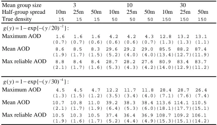
tendency to set the cutpoint too small, which can lead to positive bias (Fig. 1). However, if groups are missed whose centres are inside the selected cutpoint, negative bias will occur. It is difficult to ensure a balance between these biases.
AOD Methods
174 175 176 177 178 179 180 181 182 183 184 185 186 187 188 189 190 191 192 193 194 195 196 197 198 199
AOD tended to overestimate density of primates while the maximum AOD tended to underestimate density. He then defined a ‘maximum reliable AOD’ – the distance at which the frequency of sightings falls when plotting AOD against number of sightings. This too was used as an estimate of the strip half-width. In each case, only AODs less than the estimated half-width were included in the density estimate (Struhsaker, 1981). We can find no published results that show that he compared methods based on perpendicular distances and AODs measured in the field.
Assumptions
Beyond the assumption that the selected truncation distance results in a complete count of primate groups within that same distance of the line, assumptions are never explicitly stated for the modified Kelker method and its AOD variants. In fact, there is no coherent framework under which the methods can be justified, so that it is not possible to specify a full set of assumptions, as will be seen below.
Problems
The method, like the Kelker strip, is subjective when the ‘maximum reliable AOD’ is used, so that different analysts may select different truncation distances, and estimation is sensitive to the choice. When there is a subjective element in the analysis, and estimation is sensitive to the subjective choice, it is good practice for assessments of the performance of the method based on populations with known density to be performed blind – that is, the analyst should be unaware of the true density when generating estimates.
200 201 202 203 204 205 206 207 208 209 210 211 212 213 214 215 216 217 218 219 220 221 222 223
do not reflect spatial variation (so-called pseudo-replication, Hurlbert, 1984). Variance could be estimated as for strip transect sampling, although this fails to incorporate uncertainty in estimating the strip width.
However, there is a more serious problem with these methods, in that their conceptual framework is erroneous. The methods confuse a probability density function with a detection function. When a histogram is plotted, showing frequencies of detections by distance intervals, then the histogram, if rescaled so that the total area of the histogram bars is unity, provides an empirical estimate of a probability density function: it shows the relative frequencies of detections by distance. By contrast, the detection function is the probability of detecting a group, as a function of distance of that group from the line or, for AOD methods, from the observer. When perpendicular distances from the line are used, the two functions have the same shape (Buckland et al., 2001:53), so that the histogram may be used for example to assess the perpendicular distance at which probability of detection starts to fall. However, if AODs are used, this is no longer the case (see e.g. Buckland et al., 2001:148). The point at which frequencies start to fall does not correspond with the point up to which probability of detection is certain. To illustrate this, we simulated data using the hazard-rate model
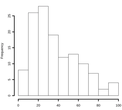
for the detection function (Fig. 2), where is the probability of detecting an animal group whose centre is at perpendicular distance y from the line. Groups had mean size of three, and half the group spread was 10m. (Full details are given in the simulation study section below.) We show a histogram of simulated AODs (Fig. 3). The ‘maximum reliable AOD’ might be taken as 30m or 40m, depending on the judgement of the analyst, but detectability starts to fall away at around 10m (Fig. 2). The effect is substantial; over 60% of groups are undetected at 30m, and nearly 80% at 40m. In other words, for these } ) 20 / ( exp{ 1 )
(y = − − y −2 g
)
(y
224 225 226 227 228 229 230 231 232 233 234 235 236 237 238 239 240 241 242 243 244 245 246 247 248 249
values of the maximum reliable distance, we can expect underestimation of density by over 60% (30m) or nearly 80% (40m).
This flaw in the method is self-evident if you consider what is being done. For example, Hassel-Finnegan (2008) report in their Fig. 2 an estimate of 55m, estimated from AODs, up to which detection is considered to be certain for white-handed gibbons Hylobates lar carpenteri. However, of 155 detections, 141 of these were not detected until they were closer to the observer than 55m. Indeed, the median AOD is under 35m. If animals at 55m were certain to be detected, then AODs of less than 55m should not be observed – as the observer approaches an animal, then it will be detected at the certain detection distance of 55m, if not at a greater distance.
Marshall et al. (2008), while acknowledging that the method lacks a mathematical basis, state erroneously: ‘Because sighting distance is used rather than distance to transect, the pattern of decline with distance is a true detection function.’ This is not the case (Fig. 3). Hence their belief that the method should be used when other methods fail lacks credibility.
There is a further inconsistency in the method, when the histogram is used to identify the distance up to which detection is certain. AODs are used to estimate (erroneously) this distance. However, this is then assumed to be the half-width of a strip centred on the line, rather than the radius of a circle centred on the observer. It is also used to truncate detections whose AODs are larger. Suppose we use 55m as the truncation AOD as in Hassel-Finnegan et al. (2008). A group that is detected when still 80m away, but which is located on the line, is therefore excluded from the count – but its location is right at the centre of the strip to which the count supposedly relates.
250 251 252 253 254 255 256 257 258 259 260 261 262 263 264 265 266 267 268 269 270 271 272 273 274 275
observer to be the location of the first detected animal of a group: the upward bias generated by this strategy might cancel with the downward bias of the modified Kelker method. There is no assurance that the biases will cancel in general.
Review of Papers that have Assessed AOD Methods
Struhsaker (1981) proposed use of the modified Kelker method on the basis that it gave rise to the least biased estimates of density of red colobus monkeys Piliocolobus oustaleti. However, the reason for overestimation of density in his study is evident from the following quote: ‘… nearly 40% of the 166 sightings of red colobus were over the census transect and were scored as zero meters from the trail …’ He does not clarify how distances were measured in the field, but as all groups ‘over the census transect’ were recorded as being at zero distance, we can infer that distance of the nearest animal to the transect was recorded, with predictable overestimation of density; any attempt to salvage density estimates from such poor distance data will inevitably be subjective and ad hoc. (Another possibility is that the position of the line was not well-defined, so that any animal or animal group that was close to the line was simply recorded as on the line.)
276 277 278 279 280 281 282 283 284 285 286 287 288 289 290 291 292 293 294 295 296 297 298 299 300 301
Chapman et al. (1988) used just 5 transects, subjectively placed. Their known populations comprised just a single group of each of two species (white-headed capuchin Cebus capucinus and mantled howler monkey Alouatta palliata) in Costa Rica. They used six different methods of measuring distances: ‘the mean, maximum and reliable perpendicular distance from the transect to the animal first sighted and the mean, maximum and reliable distance from the observer to the animal.’ Thus all six methods were prone to bias by assuming that the first animal sighted was at the centre of the group. The authors did not quantify the precision of their estimates, and did not define what a ‘reliable’ distance is (there is not a unique definition of it in the literature). Their estimates show poor performance of all methods, with no clear winner, yet they come down heavily in favour of methods based on AODs on the grounds that ‘sightings that occur directly over the transect or at a steep angle to it, are likely to cause bias.’ They do not clarify why. They also claim that the ability of the observer to estimate perpendicular distance will be limited when the terrain is rough, which in our view is not a compelling reason for using the wrong distance. Analyses presented in the paper do not in fact support the use of AOD methods; rather, misunderstanding of the methods has resulted in their recommendation to use it.
half-302 303 304 305 306 307 308 309 310 311 312 313 314 315 316 317 318 319 320 321 322 323 324 325 326 327
width from a histogram, coupled with adding half the group spread to this distance (Whitesides et al., 1988). Uncertainty over true density complicated assessment of the methods, and they drew no firm conclusions on which method was best.
Fashing and Cords (2000) analysed data on two species (black-and-white colobus Colobus guereza and blue monkey Cercopithecus mitis) in Kenya. They estimated true densities based on home range data primarily on five groups and three groups respectively, although data from additional groups were also used. The ‘design’ was of a single non-random transect, placed along trails. They estimated precision from variation in repeat runs along the same transect. They estimated transect width using a) the maximum reliable AOD; b) the maximum reliable perpendicular distance; and c) the maximum reliable perpendicular distance with the addition of half the group spread, as recommended by Whitesides et al. (1988). They also used the shape-restricted estimator of Johnson and Routledge (1985) (a type of perpendicular distance detection function estimator that is seldom used). For both species, the method based on perpendicular distances, together with the half-group spread correction, gave estimates closest to the true density. The shape-restricted estimator performed particularly poorly.
328 329 330 331 332 333 334 335 336 337 338 339 340 341 342 343 344 345 346 347 348 349 350 351 352 353
the true density, while the modified Kelker method gave estimates very slightly under the true density. However, given the lack of replication (a single line, and a single group of each species), it seems that little can be inferred from these results. Hassel-Finnegan et al. (2008) quote the papers of Chapman et al. (1988) and Fashing and Cords (2000) to support their contention that analyses based on AODs closely match true densities, while those based on perpendicular distances overestimate. However, the results of neither paper support this conclusion.
All of the above comparisons are based on studies where true density is established by studying a small number of habituated groups, and estimating the size of their home range. There are several reasons why there might be bias in these ‘true’ densities. For example home ranges of groups may partially overlap, and because the transects in these studies are positioned subjectively, they may sample parts of the home range that are favoured or avoided by the habituated group, leading to a mismatch in the densities being estimated by the two approaches. This is exacerbated when the sampled strip(s) extend beyond the home range(s) of the habituated group(s), into other home ranges. Further, lone males are not included in densities obtained from home range studies, so that density might be expected to be lower as assessed by this method than that obtained by appropriate application of line transect sampling methods. In the case of a population of grey-cheeked mangabeys Lophocebus albigena in Uganda (Olupot and Waser, 2005), Olupot (pers. comm.) estimates that around 30% of males are solitary, corresponding to around 8% of the total population.
354 355 356 357 358 359 360 361 362 363 364 365 366 367 368 369 370 371 372 373 374 375 376 377 378
census periods (1975-76 and 1996 Struhsaker; 1997-98 Lwanga; and 1996 Mitani). They also used a single transect, which formed the shape of a square route. The authors found great variation in the estimation of AOD between the three of them, showing that each observer would estimate a very different maximum reliable sighting distance and that the shape of the sighting distributions differed significantly. They therefore could not use the modified Kelker method to compare densities between years and resorted to comparing encounter rates of primate groups per kilometre walked. Variation between observers with the modified Kelker method eliminates any possibility of comparison unlike standard perpendicular distance methods where a probability of detection can be computed for each observer to allow comparisons to be made (Marques et al., 2007).
379 380 381 382 383 384 385 386 387 388 389 390 391 392
Simulation Study
Simulating Populations and Samples
To assess how different methods perform, we simulated data from populations of known density. This is intentionally an idealized study, with a large sample of lines systematically spaced with a random start, with certain detection of animals on the line, no responsive movement, and no measurement error in distances. If methods perform poorly here, they can certainly be expected to in real studies. For simplicity, we assumed a rectangular survey region, 20km long and 5km wide. We placed 25 transects in the region, each 5km long, spaced 800m apart.
True number of groups in the survey region was 500, randomly spread through the region with a uniform density. Mean group size was 3, 10 or 30 animals, so that total population size was 1500, 5000 or 15000, corresponding to 15, 50 or 150 animals per square kilometre. We assigned the animals to the 500 groups by first assigning a single animal to each group. We then generated a random number for each remaining animal from a continuous uniform distribution on (0,500p), with p=0.75. We raised this number to the power , and rounded up to the next integer; the resulting value defined the group to which the animal was assigned. This ensures greater variation in group size than would occur if all groups had the same expected size (corresponding to ), but the expectation of mean group size was 3, 10 or 30, as required. We assigned the position of each animal in a group at random within a circle of radius
393 394 395 396 397
p
/ 1
1 =
p
ρ, centred at the assigned group location, with
398
=
ρ 10, 25 and 50m. All group centres fell within the survey region, but individual animals could be assigned a location outside the survey region. To avoid the complication of partial sampling of groups straddling the boundary, we extended sampling into a bufferzone, to allow the whole group to be sampled. We did not count effort (i.e. length of transect) in the bufferzone; this does not create bias 399
404 405 406 407 408 409 410
because the additional sightings compensate for the ‘missing’ sightings that would have occurred had groups been simulated whose centres were outside the study region, but which straddled the boundary.
Hayes and Buckland (1983) developed a hazard-rate model of the detection process. Their model is useful here to simulate the detection process as the observer approaches a group of animals. In this study, we initially simulated whether or not an animal was detected independently of other animals in a group. We assumed a hazard function of the form k(r)=ar−b,with b=3 and b=5, where r is distance between the animal and the observer. If the observer has not yet detected an animal at distance r, then is the probability that the animal is detected as the observer advances a small distance dx along the line. Given the above form for , we can derive the detection function , which is the probability that an animal at distance y from the line is
detected: . We chose (
411 412 413 414 415 dx r k( )
) (r k ) (y g } ) / ( exp{ 1 )
(y = − − y c −(b−1)
g c=20, b=3), for which ,
and ( , ), for which
400 = a 416 30 =
c b=5 a=1215000. These two detection functions are shown (Fig. 2). To mimic the enhanced probability of detecting animals in a group once the first animal of the group has been detected, we identified all groups for which at least one animal was detected, and simulated a second ‘pass’ to search for undetected animals in the group, again using a hazard-rate detection function, but with the scale parameter c increased by 50% ( for scenarios with
417 418 419 420 421 30 =
c b=3, and c=45 when b=5). 422
423 424 425 426
427 428 429 430 431 432 433 434 435 436 437 438 439 440 441 442 443 444 445 446 447 448 449 450 451 452
Estimating Densities
For each combination of mean group size, group spread, true density and detection function, we simulated 100 populations, and surveyed each once. We applied the following analysis methods.
1. The modified Kelker method, based on mean AOD, where AOD for each detected group is the distance of the first detected animal from the group. We took the mean AOD as an estimate of the strip half-width, and the mean of recorded sizes of detected groups as an estimate of mean group size in the population.
2. The modified Kelker method, based on maximum AOD, where AOD for each detected group is the distance of the first detected animal from the group. We took the maximum AOD as an estimate of the strip half-width, and the mean of recorded sizes of detected groups as an estimate of mean group size in the population.
3. The modified Kelker method, based on maximum reliable AOD, where AOD for each detected group is the distance of the first detected animal from the group. We grouped AODs into 10m bins, and estimated the half-width of the strip by starting at the bin closest to the line (0-10m), and identifying the first bin for which the count was at most one half of the mean count for preceding bins. If for example the mean count in the first four bins was 10.5, and the count for bin 5 (40-50m) was 5, then the strip half-width was taken to be 40m, and detections at a greater distance were excluded from the analysis. We estimated mean group size in the population by the mean of recorded sizes of detected groups.
Results
453 454 455 456 457 458 459 460 461 462 463 464 465 466 467 468 469 470 471 472 473 474 475 476 477
detection function. This finding is consistent with the finding by Mitani et al. (2000), that density estimates were not comparable across observers. The bias is especially large for method 1, the maximum AOD method (-90.7% and -75.7% for the two detection functions). For method 2, bias was -42.3% for the first detection function and -25.1% for the second. The corresponding values for method 3 were -43.9% and -28.2%.
These biases are not fully explained by bias in recorded group sizes (Table 2). Interestingly, although bias in recorded group size increases both with mean group size and with group spread, for methods 2 and 3, bias in density estimates within a method and detection function is largely independent of mean group size and group spread. However, as the bias is not consistent across different detection functions, it suggests that neither method gives a reliable estimate of relative density.
The bias is also not attributable to recording distances to the first detected animal, rather than to the group centre. Using measurements to group centres, AODs would increase, resulting in larger estimated strip widths, and reduced densities, so that bias would be even larger.
Because the methods have no coherent mathematical framework, it is not possible to identify the causes of bias, as there are no coherent assumptions that we can assess.
Discussion
478 479 480 481 482 483 484 485 486 487 488 489 490 491 492 493 494 495 496 497 498
For methods based on selecting a single animal, and using the distance to it as the distance to the group centre, there is some ambiguity in the literature about whether the selected animal is the first animal detected or the closest animal. In general, the two are not the same individual. In our simulations, we assumed that it is the first animal detected. Struhsaker (1981) recorded 40% of detected groups as being on the line, which suggests that he used the distance of the closest animal to the line. Alternatively, if his transect was along trails, it may be that animals directly above the line were the first to be detected, because they were more visible.
We conclude that AOD methods as used by primatologists are conceptually flawed; the resulting estimates should not be treated as estimates of absolute density. Whether they are acceptable estimates of relative density depends on many factors. Estimates are unlikely to be comparable across different observers (Mitani et al., 2000) or habitats for example. Estimating primate abundance is often difficult compared with many other taxa, as the animals often reside in hard-to-access, low-visibility areas and are often clustered, cryptic and highly mobile. Nevertheless, more reliable estimates of abundance are potentially possible by combining good survey design with better field and analytic methods (Buckland et al., in review).
499 500 501 502 503 504 505 506 507 508 509 510 511 512 513 514 515 516 517 518 519 520 521 522 523
References
Brugiere, D., & Fleury, M. -C. (2000). Estimating primate densities using home range and line transect methods: a comparative test with the black colobus monkey Colobus satanus. Primates, 41, 373-382.
Buckland, S. T., Anderson, D. R., Burnham, K. P., Laake, J. L., Borchers, D. L., & Thomas, L. (2001). Introduction to Distance Sampling. Oxford: Oxford University Press.
Buckland, S. T., Anderson, D. R., Burnham, K. P., Laake, J. L., Borchers, D. L., & Thomas, L. (Eds). (2004). Advanced Distance Sampling. Oxford: Oxford University Press.
Buckland, S. T., Plumptre, A. J., Thomas, L., & Rexstad, E. A. (in prep.). Design and analysis of line transect surveys for primates.
Chapman, C., Fedigan, L. M., & Fedigan, L. (1988). A comparison of transect methods of estimating population densities of Costa Rican primates. Brenesia, 30, 67-80.
Defler, T. R., & Pintor, D. (1985). Censusing primates by transect in a forest of known primate density. Int J Primatol, 6, 243-259.
Fashing, P. J., & Cords, M. (2000). Diurnal primate densities and biomass in the Kakamega Forest: an evaluation of census methods and a comparison with other forests. Am J Primatol, 50, 139-152.
Hassel-Finnegan, H. M., Borries, C., Larney, E., Umponjan, M., & Koenig, A. (2008). How reliable are density estimates for diurnal primates? Int J Primatol, 29, 1175-1187. Hayes, R. J., & Buckland, S. T. (1983). Radial distance models for the line transect method. Biometrics, 39, 29-42.
524 525 526 527 528 529 530 531 532 533 534 535 536 537 538 539 540 541 542 543 544 545 546 547 548 549
Hurlbert, S. H. (1984). Pseudoreplication and the design of ecological field experiments. Ecological Monographs, 54, 187-211.
Johnson, E. G., & Routledge, R. D. (1985). The line transect method: a nonparametric estimator based on shape restrictions. Biometrics, 41, 669-679.
Kelker, G. H. (1945). Measurement and Interpretation of Forces that Determine Populations of Managed Deer. PhD thesis, University of Michigan.
Marques, T. A., Thomas, L., Fancy, S. G. and Buckland, S. T. (2007). Improving estimates of bird density using multiple covariate distance sampling. The Auk, 124, 1229-1243.
Marshall, A. R., Lovett, J. C., & White, P. C. L. (2008). Selection of line-transect methods for estimating the density of group-living animals: lessons from the primates. Am J Primatol, 70, 1-11.
Mitani, J. C., Struhsaker, T. T., & Lwanga, J. S. (2000). Primate community dynamics in old growth forest over 23.5 years at Ngogo, Kibale National Park, Uganda: implications for conservation and census methods. Int J Primatol, 21, 269-286.
Olupot, W., & Waser, P. M. (2005). Patterns of male residency and intergroup transfer in gray-cheeked mangabeys (Lophocebus albigena). Am J Primatol, 66, 331-349.
Plumptre, A. J., & Cox, D. (2006). Counting primates for conservation: primate surveys in Uganda. Primates, 47, 65-73.
Struhsaker, T. T. (1975). The red colobus monkey. Chicago: University of Chicago Press.
Struhsaker, T. T. (1981). Census methods for estimating densities. In National Research Council, Techniques for the Study of Primate Population Ecology (pp. 36-80). Washington: National Academy Press.
550 551 552 553 554 555
design and analysis of distance sampling surveys for estimating population size. J App Ecol.
Figure legends
Fig. 1. Shown here are two datasets, both generated from a detection function with certain detection out to 40m, and rapidly declining detection probability at larger distances. When by chance there are more detections close to the line, visual inspection of the data leads to selection of a smaller cutpoint for the Kelker method; 20m in this example. When there are more detections close to 40m, the cutpoint is likely to be set at 40m. If we fix the cutpoint in advance, at either 20m for both analyses or 40m, we expect unbiased estimates of density, but if we use 20m for the first analysis and 40m for the second analysis, we overestimate density on average. Dashed lines: mean count with truncation at 40m. Dotted lines: mean count with truncation at 20m.
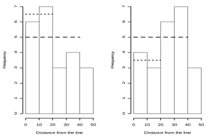
Fig. 2. The detection functions used in the simulation study. Note that these detection functions apply to each individual animal; the probability that at least one animal of a group will be detected will be larger than shown here – substantially so for large groups.
The solid line is and the dashed line
.
} ) 20 / ( exp{ 1 )
(y = − − y −2 g
} ) 30 / ( exp{ 1 )
(y = − − y −4 g
Table 1. Mean (standard deviation in parentheses) of density estimates for the three methods of estimation.
Mean group size 3 10 30
Half-group spread 10m 25m 50m 10m 25m 50m 10m 25m 50m True density 15 15 15 50 50 50 150 150 150
} ) 20 / ( exp{ 1 )
(y = − − y −2
g :
Maximum AOD 1.6 1.6 1.6 4.2 4.2 4.3 12.8 13.2 13.1 (0.7) (0.7) (0.6) (0.6) (0.6) (0.7) (1.3) (1.3) (1.1)
Mean AOD 8.6 8.5 8.3 29.6 29.2 29.0 85.5 88.2 87.4 (1.9) (1.7) (1.5) (5.2) (4.0) (4.0)(13.4)(12.7)(11.9)
Max reliable AOD 8.8 8.4 8.4 28.7 28.2 27.6 80.9 83.4 83.7 (2.1) (1.7) (1.6) (5.3) (4.3) (4.2)(14.0)(12.9)(11.2)
} ) 30 / ( exp{ 1 )
(y = − − y −4
g :
Maximum AOD 4.5 4.5 4.7 12.2 11.7 11.8 28.4 28.7 26.4 (1.3) (1.5) (1.2) (3.5) (3.4) (4.0) (7.1) (7.6) (7.4)
Mean AOD 10.7 10.8 11.0 39.2 38.3 38.4 113.6 114.1 110.5 (2.1) (1.7) (1.9) (6.4) (5.3) (6.0)(18.1)(17.7)(15.1)
Table 2. Estimates of mean group size: sample mean (standard error in parentheses) of recorded group sizes within w of the line.
Mean group size 3 10 30
Half-group spread 10m 25m 50m 10m 25m 50m 10m 25m 50m }
) 20 / ( exp{ 1 )
(y = − − y −2
g :
2.65 2.56 2.33 6.46 6.27 5.68 14.28 14.31 13.29 (0.20)(0.19)(0.14)(0.39)(0.36)(0.33)(0.89)(0.97)(0.82)
} ) 30 / ( exp{ 1 )
(y = − − y −4
g :
Fig. 1. Shown here are two datasets, both generated from a detection function with certain detection out to 40m, and rapidly declining detection probability at larger distances. When by chance there are more detections close to the line, visual inspection of the data leads to selection of a smaller cutpoint for the Kelker method; 20m in this example. When there are more detections close to 40m, the cutpoint is likely to be set at 40m. If we fix the cutpoint in advance, at either 20m for both analyses or 40m, we expect unbiased estimates of density, but if we use 20m for the first analysis and 40m for the second analysis, we overestimate density on average. Dashed lines: mean count with truncation at 40m. Dotted lines: mean count with truncation at 20m.
Distance from the line
F
re
que
nc
y
0 10 20 30 40 50
0123
4
567
Distance from the line
F
re
que
nc
y
0 10 20 30 40 50
0123
4
Fig. 2. The detection functions used in the simulation study. Note that these detection functions apply to each individual animal; the probability that at least one animal of a group will be detected will be larger than shown here – substantially so for large groups.
The solid line is and the dashed line
.
} ) 20 / ( exp{ 1 )
(y = − − y −2 g
} ) 30 / ( exp{ 1 )
(y = − − y −4 g
0 20 40 60 80 100
0
.0
0
.2
0
.4
0
.6
0
.8
1
.0
Distance y from the line
D
e
te
c
ti
on f
u
nct
ion g(
Fig. 3. Histogram of AODs simulated from the hazard-rate model of the detection process, . g(y)=1−exp{−(y/20)−2}
Animal-to-observer distance
F
requency
0 20 40 60 80 100
0
5
1
0
15
20