http://research-repository.st-andrews.ac.uk
The digital repository of research output from the University of St Andrews Version This is an author version of this work which may vary slightly from the
published version.
Date Deposited in repository on 17 June 2011
Access
rights This work is made available online in accordance with publisher policies.Published version is copyright © 2008 by the Society for Marine Mammalogy. To see the final definitive version of this paper please visit the publisher’s website.
Citation for published version:
Estimating the Barents Sea polar bear subpopulation size
J. Aars1, T. A. Marques2, S. T. Buckland2, M. Andersen1, S. Belikov3, A. Boltunov3, Ø.
Wiig4.
1
Norwegian Polar Institute, N-9296 Tromsø, Norway;2Centre for Research into
Ecological and Environmental Modelling, University of St Andrews, St Andrews KY16
9LZ, Scotland;3All-Russian Research Institute for Nature Protection, 113628 Moscow,
Russia;4Natural History Museum, University of Oslo, N-0318 Oslo, Norway.
Running headline:
Estimating the Barents Sea polar bears
Correspondence: Jon Aars, Norwegian Polar Institute, Polar Environmental Centre, 9296
Abstract
A large scale survey was conducted in August 2004 to estimate the size of the Barents Sea
polar bear subpopulation. We combined helicopter line transect distance sampling surveys
in most of the survey area with total counts in small areas not suitable for distance
sampling. Due to weather constraints we failed to survey some of the areas originally
planned to be covered by distance sampling. For those, abundance was estimated using a
ratio estimator, in which the auxiliary variable was the number of satellite telemetry fixes
(in previous years). We estimated that the Barents Sea subpopulation had approximately
2650 (95% CI approx 1900 to 3600) bears. Given current intense interest in polar bear
management due to the potentially disastrous effects of climate change, it is surprising
that many subpopulation sizes are still unknown. We show here that line transect sampling
is a promising method for addressing the need for abundance estimates.
Key-words: Helicopter surveys, distance sampling, line transects, polar bear, Barents Sea,
Introduction
Polar bears were heavily hunted during the first half of the 20thcentury all over the Arctic.
In the early 1960’s scientists and managers from the five polar bear nations (Canada,
Denmark (Greenland), Norway, Soviet Union, and USA) started to work on an
international plan for conservation of polar bears. The outcome of this work was the
international “Agreement on the Conservation of Polar Bears”, signed in 1973 (see
Prestrud and Stirling 1994). One central statement in the agreement is that “Each
Contracting Party... shall manage polar bear populations in accordance with sound
conservation practices based on the best available scientific data.” Monitoring change in
population size is the most direct method for monitoring population status. The
importance of using scientifically derived population estimates in the management of
polar bears has recently been stressed (Wiig 2005, Aarset al. 2006).
The Barents Sea polar bear subpopulation, shared between Norway and Russia, has not
been harvested since 1956 in Russia and since 1973 in Norway (Prestrud and Stirling
1994). Persistent pollutants (Bernhoftet al. 1997, Norstromet al. 1998, Andersenet al.
2001), climate change (Derocher 2005), and oil development (Downing and Reed 1996,
Isaksenet al. 1998) are possible threats to the subpopulation. No meaningful estimate of
the size of the subpopulation based on any study that covers the whole area in question
has been available until now (Wiig and Derocher 1999). In the early 1980’s, Larsen
(1986) suggested that the Barents Sea polar bear subpopulation size was between 3000
and 6700 (dependent on subpopulation definition). This was based on data from multiple
sources including den counts and spatially restricted, non-random air surveys, and
With recent statistical developments, distance sampling is one of the most widely used
methods for estimating animal abundance (Bucklandet al. 2001), and is today considered
to be more cost efficient than capture-recapture to achieve a given precision (Borcherset
al. 2002), in particular for populations occurring at low densities over large areas. Wiig
and Derocher (1999) advocated a line transect study for the Barents Sea area to estimate
the subpopulation size, due to the large area and the lack of logistical bases needed for
capture-recapture based estimates. Pilot studies on polar bears in Norway and the United
States have examined the applicability of aerial surveys over sea ice, employing both strip
transects and line transects. However, density estimates have not been extended to
subpopulation estimates due to small sample sizes, restricted coverage, and
methodological uncertainties (Wiig and Bakken 1990, Wiig 1995, Manlyet al. 1996, Wiig
and Derocher 1999, Evanset al. 2003).
Wiig and Derocher (1999) reviewed aerial survey attempts in the Barents Sea, comparing
them with mark-recapture techniques, and concluded that line transect surveys would be
the most economical and effective means to estimate and monitor the polar bear
subpopulation size. In the present paper we report on a large-scale line transect survey of
polar bears that was conducted in the Barents Sea in August 2004.
Materials and Methods
STUDY AREA
The aerial survey was conducted between 26thof July and 1stof September 2004, in the
Barents Sea area (Fig. 1). The Barents Sea polar bear subpopulation has earlier been
defined as the animals occupying the area between longitudes of 10°E and 60°E, and
Russia) archipelagos (Wiig and Derocher 1999), but we chose to include both the whole
of Franz Josef Land, and areas extending slightly west of 10°E and east of 60°E allowing
parallel survey lines extending north from the ice edge (Fig. 1). The latitudinal boundaries
vary seasonally with the sea ice extent, and in August bears are not found south of about
76° 30’. In 2004, there was less sea ice around the islands than in most recent years, and
the sea ice edge was in most places further north with a very distinct edge, and very
stationary during the period of survey. Movements of bears are lowest at the time of year
the survey was conducted (Mauritzen et al. 2003), and they are not expected to be
directional as in spring or late autumn when bears move between hunting and denning
areas, or earlier in summer when sea ice distribution changes considerably.
SURVEY DESIGN
Before the survey was conducted, we used capture and satellite tracking data, as well as
historical knowledge, to plan the survey design. Bears could be encountered either on or
around islands (land, glaciers or on land fast sea ice) or in the pack ice in the Arctic Basin
(hereafter termed pack ice or PI). The Svalbard areas were considered to be either: a0areas
were bears were unlikely to be encountered in late summer, or apareas were there could
be polar bears present. Areas in category a0were excluded from the survey (bear density
assumed 0). For areas where polar bears could be present, a further sub-division was
made: apcsmall areas not well suited for line transect sampling, with expected high
densities of polar bears and apdareas well suited for line transect sampling, mostly with
presumed intermediate densities. Areas apcwere either small islands or relatively narrow
strips of land between fjords and steep cliffs, and were free of snow. It was therefore
Areas apd, together with areas of sea ice and all the islands of FJL, were surveyed using
line transect sampling.
The distance sampling survey design for areas apdwas created using the survey design
engine in Distance (Thomas et al. 2006). Line spacing was 3km for all islands and sea ice
areas. This spacing was chosen according to flight hours and survey time available. In
different sub-areas line orientation was determined to minimize transects along shore
areas, placing lines perpendicular to any potential density gradients. The line transect
coordinates were imported into Arcview (www.ESRI.com), and from there uploaded into
a GPS unit that was used in the helicopter during the survey.
When transects were flown over land and glaciers, they were continued over the sea
wherever there was ice (fast ice or drift ice) present. Around Svalbard, there was virtually
no sea ice left. Only 41 km of transect line was flown to cover what was left, and no bears
were observed. Thus we ignored these transects in the analyses (bear density assumed 0).
Also some very open drift ice (Fig. 1) was not covered due to safety considerations.
While most of the land areas were surveyed according to the planned 3 km line spacing
pattern, the line spacing of glaciers on FJL was often changed. Because fog often
prevented flying across glaciers, every 2ndor 3rdline were flown (Fig. 1), resulting in
respectively 6 or 9km line spacing. In Svalbard, the coverage on glaciers was even more
sporadic than on FJL (Fig. 1), because of almost continuous dense fog over the glaciers
For the PI area, 89 transect lines 9 km apart were laid roughly northward from the ice
edge, with the most western and eastern lines running from respectively 9°39.4’E,
81°26.0’N to 6°13.2’E, 82°30.3’N and 60°28.4’E, 81°54.5’N to 63°48.6’E, 82°41.0’N
(see Fig. 1). These lines extended 185km north from the ice edge. Due to time and
fog-induced safety constraints, 17 lines were not covered, and most surveyed lines were
shorter than 185km (Fig. 1).
For analysis we considered 7 geographic strata, based on the interaction of administrative
regions (Russia and Norway) and habitats (Pack Ice, Land, Glacier and Sea Ice, the latter
around islands, only in Russia) (Fig. 1).
FIELD METHODS
Two one-engined helicopters (Eurocopter AS350 Ecureuil) were used for flying total
counts and line transects. One helicopter was stationed at Longyearbyen, Svalbard,
covering the Svalbard archipelago from 26th– 31stof July, and 14th–26thof August. The
second helicopter was stationed onboard the research vessel RV Lance (from 1st– 31stof
August) operating along the ice edge in the Barents Sea and in the FJL archipelago area.
The helicopters operated with four observers including the pilot. The two observers in the
front seats focused on the transect line in front of the helicopter, while the two rear
observers focused to each side of the helicopter further away from the transect line, but
with some overlap with the front observers’ search areas. The helicopters generally flew at
200 feet (61 m) above ground and at 100 knots speed (185 km/hour). Due to weather
conditions, other combinations of altitude and speed were used for one transect at the PI,
The speed and altitude for flying were chosen after a pilot study (Aars et al., unpublished
data) to ensure that the probability of observing a bear on the transect line, g(0), was
maximized. We tested different altitudes and varying speed and found that a speed of 185
km/hour and altitude of 60 m was optimal.
The predetermined transect lines were flown using the GPS unit to which the survey
design had been previously uploaded. This GPS unit also recorded a detailed track of the
actual flight path. Details can be found in Marques et al (2006). The helicopter that
operated from the research vessel in the Russian area and along the PI had two complete
survey teams including two pilots, to allow transects to be flown almost continuously in
periods of good weather.
When single transect lines covered different habitat types (land, glacier, fast ice, drift ice),
each stretch of one habitat type was categorized as a section. For analysis, all sections of
the same habitat type along a single line were then pooled (e.g. a flown line with 10 km
ice + 10 km land + 10 km ice was considered as 2 transects, 1 with 20 km ice and 1 with
10 km land). For each bear observation, habitat structure was recorded as a covariate and
scored as: 1 = relatively flat surface with only minor or no structure of the size that could
make it difficult to spot a polar bear; 2 = habitat with some structure that could make it
harder to spot a bear in the area (e.g. some screwed sea ice or crevasses on glaciers); 3 =
major structures present that make it considerably more difficult to detect polar bears (e.g.
heavily screwed sea ice).
We used distance sampling (DS) as described by Bucklandet al. (2001, 2004) to estimate
bear abundance.
For populations which potentially occur in well defined clusters, like polar bears, the
perpendicular sighting distances to the center of detected clusters allows the modeling of a
detection function, g(y), which represents the probability of detecting a cluster, given that
it is at distance y from the transect line (Bucklandet al. 2001). Parametric models are
assumed for this detection function, and their parameters estimated via maximum
likelihood, with the possibility to include adjustment terms for fit improvement. The
probability of detecting a cluster in the covered areas, P, is the mean value of the detection
function with respect to the available distances. While conventional methods use only the
perpendicular distance y for detection function modeling, multiple covariate distance
sampling (MCDS) extends the methods to include additional covariates z to help model
the detection function. The scale parameter of the detection function becomes a function
of these additional covariates (Marques and Buckland 2003). If MCDS is used, the
probability of detection associated with cluster i, Pa(zi) (i=1,2,…,n, where n is the total
number of detected clusters) is conditional on the corresponding covariate values zi. An
estimate of cluster abundance in the covered area (corresponding to the covered strips of
width 2w, i.e. extending a distance w either side of the lines) of sizeais then obtained by
(e.g. Marques and Buckland 2003)
n
i a i
cs
z P N
1 ˆ ( )
1
ˆ .
To estimate animal abundance, this estimate can be multiplied by an estimate of mean
Given an appropriate random sample of lines (see Strindberget al. 2004 for design
details), one can extrapolate the results obtained in the covered area, based on the design
properties, to the wider survey region. In our case, purely design-based extrapolation was
not possible for the entire PI because it was not possible to survey all the transect lines, so
that an additional procedure was required (see below). We define the surveyed area as the
area within which a systematic sample of surveyed transects was conducted, and for
which we can estimate abundance using line transect sampling alone. Other areas within
the study region, to the north of covered strips or within the gap in survey coverage (areas
D,E and F, Fig. 1) are referred to as the unsurveyed area.
The conventional methods used in our survey rely on a set of assumptions (Bucklandet al.
2001), the most important being: (1) a large number of transects are randomly allocated in
the study area independently of the distribution of the population of interest; (2) all
animals on the line are detected with certainty (g(0)=1); (3) Animal movement is slow
with respect to observer movement; (4) Distances are measured without error. An
evaluation of the extent to which each of these was fulfilled is provided in the Discussion.
Preliminaries
Both the tracks and the waypoint files from the transects flown were downloaded to a
computer and analyzed using the program GPS Map Explorer version 2.34
(http://home.tiscali.no/gpsii/). Perpendicular distances to bear clusters required for
distance sampling analysis were obtained by calculating the shortest distance from the line
flown, as recorded by GPS, to the waypoint representing the location of the bear (or bear
Extensive plotting of detected distances, number of detections, encounter rates and cluster
sizes was done during the survey, allowing the removal of virtually all typos and
recording errors.
Analysis in Distance 5.0
The line transect data were analyzed using program Distance 5.0. (Thomaset al. 2006). A
preliminary analysis of all the data with half-normal and hazard-rate detection functions
showed a well-behaved detection function decreasing with distance and no evidence of
any major problems. Preliminary analyses showed that truncation of 5% of the largest
distances (w = 1068m) was adequate to preclude fitting spurious bumps in the tail of the
detection function, and that was the truncation used in subsequent analysis.
A number of candidate covariates were available for modeling the detection function:
habitat, structure (around the position the bear was observed), cluster size and helicopter
altitude. Habitat was a factor covariate with 3 levels, structure was considered both as a
factor with 3 levels and as a continuous covariate (with values 1, 2, or 3), and the
remaining two were continuous covariates. Their inclusion was assessed by using
minimum Akaike’s Information Criterion (AIC), and the overall fit evaluated using the
standard Chi-square, the Kolmogorov-Smirnov and the Cramér-von Mises tests available
in Distance. A priori, it was thought that altitude could reflect overall flying conditions
(since under ideal conditions the altitude would be 61m). The perception based on the
fieldwork was that cluster size would not be relevant, because clusters tend to act as single
cues. Both habitat and structure were believed to be potentially useful for modeling the
detection function. As well as testing the inclusion of cluster size as a covariate, we used
log of cluster size (e.g. Buckland et al. 2001, 73:75), to evaluate and correct for the
eventual presence of size bias. For abundance estimation, we considered a common
detection function model across strata, with density estimated by stratum conditional on
the observed covariate values.
CORRECTION FOR AREAS NOT SURVEYED
Despite the carefully planned survey design, it proved impossible to survey 17 lines in the
Russian region, leaving a gap in the coverage of the PI region between Svalbard and FJL
(see area F, Fig. 1). This was due to bad weather and related safety considerations arising
from flying a one motor helicopter in a remote area. Additionally, the average length of
the lines flown in this area was 125 km (range 43 – 232 km, Fig. 1) instead of the 185 km
planned. Rather than assuming that density in the surveyed areas could be extrapolated to
these areas, we opted for a ratio estimator. Considering boxes as described below, we used
the auxiliary variable number of telemetry fixes (from adult females, see below) within
each box, to predict the number of bears that would have been detected had the lines been
flown.
The 89 lines from the study design, including the 17 that were not covered by line
transects, were considered to be the centerlines of rectangles or ‘boxes’, each 9 km wide
(4.5 km either side of the line) and 336 km long (north from the ice edge). Each box was
divided into two, the southern portion corresponding to the surveyed centerline, and the
northern portion extending the box from where survey effort stopped to the boundary 336
km north of the ice edge (the maximum distance recorded by telemetry fixes). The 17
lines not covered by the survey in the Russian sector were divided into two; a southern
part was 244 km long ( = 336 - 92 km). Thus, the size of the study region north of the ice
edge was 269,136 km2(89 x 9 km x 336km),of which 80,839 km2(30%) was surveyed by
line transect sampling, with abundance for the remaining 188 297 km2(70%) being
estimated using the ratio estimator, as described below.
The telemetry data are well described in Mauritzenet al. (2001, 2002). Satellite telemetry
fixes have high position accuracy compared to the scale on which polar bears operate. The
telemetry accuracy was estimated to be less than 1400 meters for 92% of the positions
(Mauritzen et al, 2001). We used only positions from the period when the ice edge is
furthest north (July-September) from 44 different bears tracked between 1989 and 1999.
Only positions north of 79º N and at least 20 km from land were used (169 data points). If
more than one position was available for a given bear, only positions a minimum of 6 days
apart were used to reduce dependence between bear locations. The average distance
between 93 pairs of fixes 6 days apart in time was 57 km (SD = 28 km), and thus
relatively large compared to the distance between lines (9 km). Using standard ANOVA
(p-values > 0.1), there was no significant yearly difference in the distribution of bears
relative to the distance from the ice edge, despite the latitudinal position of the ice edge
varying substantially among years. There was also no significant difference in the distance
from the ice edge when comparing data for July plus September with data for August.
Each point was allocated to the appropriate box. As a box was defined in terms of distance
from the ice edge, a fix of say 20 km north of the ice edge in 1989 would be placed 20 km
north of the ice edge in our survey, even though the ice edge was in a different absolute
The number of bears that would have been detected if transects had been flown in the
areas not surveyed, nˆuns, was estimated using the following ratio estimator
178 73 ˆ i iuns r X
n where
72 1 72 1 i i Xi Yi rand Xi is the number of telemetry fixes within box iand Yi the number of bear groups
detected within boxiduring the survey. Notei= 1, 2,…, 72 (Fig. 1, area A+B+C)
represents boxes associated with transect lines surveyed whilei= 73, 74,…, 178 (Fig. 1,
area D+E+F) represents boxes corresponding to transect line segments not surveyed.
The estimated number of animals for the unsurveyed areas (Nˆuns) is then calculated by
s c d uns uns P P n s E N | ˆ ) ( ˆ ˆ
where the relevant quantities were obtained in the distance sampling component of the
survey, i.e.Eˆ(s)is an estimate of mean cluster size, obtained using the regression method
(Buckland, 2001: 73-75) to allow for size bias,Pˆd is estimated probability of detection of
animals that are within the truncation distance w (this is obtained as the average estimated
probability of detection within each stratum, conditional on the observed covariates in that
stratum) and Pc|sis the probability that a bear is within a distance w from the survey lines,
given that it is within the surveyed areas (= 2w/box width).
The total estimated number of bears was obtained as the sum of: (1) the estimated
numbers in the surveyed area, (2) the estimated numbers in the unsurveyed area and (3)
the numbers obtained by total counts. Although the final population estimate is made up
of 3 components (total count, surveyed areas and unsurveyed areas), the first of these does
not contribute to the variance, as by definition a total count has no variance.
To obtain estimates of variance for the estimated abundances we used a non-parametric
bootstrap (999 bootstrap resamples). Variance estimates were obtained by resampling
lines within strata, as described in Bucklandet al. (2001). In the case of the PI strata, the
336 km long transects were resampled, along with all the information contained in them
(survey data and telemetry fixes). To incorporate the variance involved in estimation for
both surveyed and unsurveyed areas, the bootstrap procedure had to be implemented
outside Distance, using software R (version 2.0.1, R Development Core Team 2004), with
Distance called from R; in this way, for each bootstrap resample, an estimate of all
random quantities involved both in the distance sampling component and the ratio
estimator component were obtained. As both detections and fixes are resampled together
within the bootstrap, no assumption of independence is made between the estimate for the
unsurveyed and surveyed areas when calculating the variance of the whole subpopulation.
Confidence intervals were obtained by the percentile method (Bucklandet al. 2001). By
bootstrapping all the information within the boxes (around each line), we ensure
comparability across the two components of estimation. As shown by Davison and
Hinkley (1997), it is theoretically superior not to bootstrap at lower levels when data are
hierarchical, hence we do not bootstrap fixes within boxes in addition to boxes. In this
way, we also avoid having to assume that fixes are independent, replacing this by the
Results
TOTAL COUNTS
A total of 31 polar bears were observed during total counts on the island of Spitsbergen.
An additional 27 bears were observed on different small and medium sized islands in
Svalbard. On Kvitøya, in the north-east of the Svalbard area, 32 bears were observed. In
addition to these observations from areas that we allocated to a total count survey, we
added six bears that were observed from RV Lance or from the helicopter in the Russian
area, in areas of loose drift ice not surveyed by line transects. Thus total counts add up to
96 bears.
LINE TRANSECTS
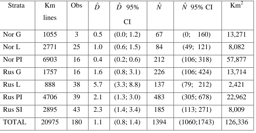
We flew 20,975 km of transect lines distributed in seven strata (Table 1). These were
considered to be 1018 independent transect units for variance estimation. A total of 189
polar bear clusters were detected. These clusters consisted of 139 lone bears and 50 adult
females with 1-3 (average 1.48) juveniles. The mean cluster size was 1.39 and the total
number of bears observed was 263.
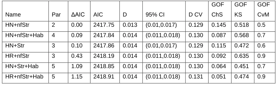
In Table 2 we present summary statistics for the candidate models considered for the
detection function, with combinations of the covariates available (models shown only if
ΔAIC<2). This table provides further reassurance on the quality of the data. Despite using
different key functions (half-normal and hazard rate) with several combinations of
covariates, the global density estimates, and corresponding associated measures of
precision, were remarkably close. Additionally none of the three absolute goodness of fit
AIC did not indicate that cluster size affected detectability (ΔAIC of 5.35 and 8.44 for the
half-normal and hazard rate models respectively). This was in accordance with field
perception. We were rarely able to distinguish between a family group and a lone animal
before we were very close, and hence at the spatial scale we were operating, bear clusters
seemed to offer a single cue independently of their size. Similarly, altitude was not
important for detection function modeling based on AIC, and hence was subsequently
ignored in the analysis.
Overall, conditional on the covariates, the half-normal key function was usually more
parsimonious than the hazard rate. Although the model with lowest AIC included only
structure as a covariate, we opted to use the next best model (ΔAIC=0.1), which included
the habitat covariate, for further inference. This was justified because we were interested
in estimation over different strata with considerably different habitats, and from the field
there was a clear perception that the detection process was different in different habitat
types.
Fig. 2 shows the distribution of observed detection distances in different habitats and
areas. Similar trends across strata made it possible to fit the half-normal detection function
to all strata, with habitat and structure as covariates.
Based on this model, we estimated bear abundance (and corresponding variances) for the
seven strata (Table 1). In total 1394 (95% CI: 1060 – 1743) bears were estimated to be in
the areas surveyed by line transects. Bear densities were much higher in Russian than
PACK ICE AREAS NOT SURVEYED
The ratio estimator was r=0.875 based on 56 observations and 64 telemetry fixes within
the PI areas covered by line transects (Fig. 3). Based on line transect data, the size bias
regression estimate of mean cluster size was 1.389, probability of detection within the
covered strip of half-width 1068m was 0.472 (Russia) and 0.442 (Norway), and the
proportion of the surveyed area covered was 1068/4500. Based on this, the number of
bears in the unsurveyed areas of the PI was estimated to be 1154 (95% CI: 659-1845, see
Table 3). The wide confidence interval obtained was partly due to the considerable spatial
variation in numbers of observations and fixes (Fig. 3).
THE TOTAL ESTIMATE
Adding the estimated numbers of bears detected by total counts, those predicted to be
within line transect survey areas and those predicted to be in unsurveyed areas of the PI,
the total is 2644 bears (95% confidence interval of 1899 - 3592).
Discussion
POPULATION ESTIMATE
We estimated the Barents Sea area to host between approx. 1900 and 3600 polar bears,
combining total counts (in small, easily surveyed areas), estimates from line transects
(over large areas) and a ratio estimator (where planned line transects were not
implemented due to safety and weather constraints). The ratio estimator approach used to
estimate abundance in areas not surveyed was the best of a number of non-ideal
alternatives, and the potential problems are discussed at length in a separate section below.
However, it is unlikely that any such survey, covering such a large area of quickly
difficult choices. We have attempted to represent the considerable uncertainty in our
estimate fairly, resulting in a rather wide confidence interval. It is assumed that the Arctic
has 19 relatively discrete subpopulations with a total of about 20,000 to 25,000 polar bears
(Aarset al. 2006). Thus, the Barents Sea subpopulation contains a considerable fraction of
the world’s population. Larsen (1986) suggested there were close to 2000 bears in the
Svalbard area, and 3000 to 6700 in the area between East Greenland and FJL in 1980.
Uncertainties around his and our estimate preclude a direct comparison. Derocher (2005)
assumed that the subpopulation had increased in size until recently.
EVALUATION OF METHODOLOGICAL ASSUMPTIONS
Total count
The relatively low number of bears observed during the total counts had little influence on
the total estimate. The failure to detect bears during these counts is therefore likely to have
negligible effect on the total abundance estimate. A few bears were also missed in areas of
very open drift ice which we did not cover by helicopter. These areas were of minor
extent, and we were fortunate to encounter a rather distinct ice edge that moved little
during the period of the survey. Larger movements of the habitat during the survey would
certainly have complicated the study. Six bears were seen from RV Lance in the FJL
region, in areas that were not covered by line transects. This was in areas with very open
water not suited for search by a one engine helicopter, and where we beforehand had
decided densities of bears would be too low to justify surveying. These observations
suggest that a considerable number of bears might have been outside the areas we
covered, and hence missed. In the absence of contemporaneous maps showing distribution
individuals in these areas. As an educated guess we believe that this might account for 100
– 200 bears.
Distance sampling
The large number of randomly allocated line transects guarantees that the design was
adequate for estimating abundance within the surveyed area. Avoidance movement before
detection would lead to a biased estimate, but is likely to generate negligible bias due to
the slow speed of the bears relative to the helicopter. Another possible problem would be
if movement away from a surveyed line generated a temporarily higher density around
neighbouring survey lines before the helicopter reached these areas. All experience we
have with polar bear behavior after disturbance is that they only react for a short period of
time when the helicopter approaches. Also, in most cases, the helicopter traveling at 185
km/hr would reach the next line before a polar bear, averaging a maximum of 4 km/hr
(Andersen et al. 2008), even when fueling or switching observational teams, and hence
this is unlikely to be a significant issue. The adequacy of the measurement procedure was
evaluated in Marqueset al. (2006), and it is reasonable to say that, at the scale we were
working, measurements were virtually error free. Therefore, it is unlikely that any of these
assumptions might have had an impact on the final estimates. The most important issue
regarding the reliability of the distance sampling population estimate is g(0). If, say 10%
of bears on the line passed undetected, then we expect our estimate to be only 90% of true
abundance (Bucklandet al. 2001). Our own perception was that bears were unlikely to be
missed on land (grey or brown background), on most areas of glaciers, and on flat, newly
formed sea ice. We think that along transects covering these habitats, g(0) was either 1 or
very close to 1. However, in some sections of transects in the PI, with heavily packed ice,
most commonly found close to open water, at the ice edge. Two polar bear observations
out of 56 in the PI area were in structure 3 habitat, and this habitat accounted for a small
proportion of the total area covered. Even if g(0) was considerably lower than 1 in
structure 3 habitat, we think that g(0) was close to 1 when averaged over all transects.
However, in accordance with recommendations from e.g. Borchers et al. (2006),
estimation of g(0) as an integral part of the study should be a priority for future similar
surveys. An eventual g(0)<1, coupled with some underestimation on the areas covered
with total counts and areas assumed to have no bears, means that, if anything, our estimate
might underestimate the subpopulation size. Nonetheless, it is our belief that provided, as
expected, g(0) was not considerably lower than 1, it is unlikely that these factors were
enough to seriously affect the quality of our estimate.
Area not surveyed
The most challenging problem resulted from the large number of transects not surveyed in
the Russian part of the PI and the restricted coverage in areas more than 90 km north of
the ice edge. Fixes of tagged females showed a tighter longitudinal spread than did
observations made in the line transect sampling, which were relatively uniform in
distribution from east to west (Fig. 3). This is presumably linked to non-random selection
of animals for tagging – tagging effort was concentrated in eastern Svalbard. Because
there was no survey effort in the north, we cannot assess whether there might be a similar
mismatch between north and south; we must assume that the tagged bears have a
representative distribution in late summer with respect to latitude, for the ratio estimator to
be approximately unbiased. The bears can walk more than 50 km in a day (Amstrup
2003). Bears tagged in Svalbard can have home range areas of many thousand square km,
2002). Thus the geographic distances per se are unlikely to limit where they can be found
along the PI. Nonetheless it is plausible to believe that bears from FJL are more
commonly found at the areas further to the east, and also that areas furthest west had more
bears from northern Svalbard rather than from eastern Svalbard. Furthermore, some bears
seen furthest west and east are likely to be from neighboring subpopulations, East
Greenland to the west and Kara Sea to the east. This would explain the mismatch of
distributions of telemetry fixes and observations from east to west (Fig. 3). This mismatch
in longitudinal distributions raises the concern about whether the ratio estimator will give
a biased estimate for the southern area (Rus Uns Fig. 1 and Fig. 3, area F) not surveyed.
The number of fixes (22) in this area predicts an average 1.3 detections per line segments
had they been covered. This is similar to what we had in the Russian sector to the west
(1.5) and east (1.3). Thus we have no indication of which direction a bias for this area
would be directed, and it seems unlikely that the bias is substantial given densities
recorded were similar in neighboring areas. It is thus of greater concern whether the
latitudinal distribution of fixes (converted to distance north of the ice edge) from several
years match with how the bears were distributed. A possible source of bias would be if
polar bears were found closer to the ice edge in years where the ice edge was located far
north. Due to the high mobility of the polar bears, it is not likely that such a relative
switch in positions relative to the edge would be caused by an increased distance from the
islands per se. However, polar bears prefer areas of more shallow water with higher
productivity (Ferguson et al. 2000). Areas further north from the ice edge have deeper
water. The ice edge in 2004 was further north than average, and thus it could be that the
ratio estimator using distributions from earlier years overestimated the number of bears in
the uncovered areas to the north. However, the failure to reveal any heterogeneity in
the position of the ice edge, means that such a bias might be small. Another indication of
this is the fact that 65 of the telemetry fixes used were from 1999, a year with a very
similar ice edge location to 2004. The average distance of fixes from the ice edge was 57
nm in 1999, only slightly shorter that that for all the 169 fixes used in the analyses (61
nm). Other potential sources of bias are the possibility that males and females or animals
at different age classes have different distributions. Little is known about this, because
telemetry data are almost exclusively available for adult females. To avoid all the possible
sources of bias, it would obviously have been preferable to have a representative sample
of collared bears with respect to both area and status, and from the year of the survey. In
our case, given that such data are not available, it might be possible to improve the
estimate during coming years by adding new information from telemetry fix data if polar
bears in the future are fitted with satellite transmitters in areas from where we currently
have low coverage (northern part of Svalbard and Russian areas).
Comparison with other studies
In our study, the average density of polar bears was 1.1 per 100 km2in the areas
surveyed by line transects (125,000 km2). In comparison, Taylor and Lee (1995) estimated
an average density of 0.4 (range 0.1 - 1.0) bears per 100 km2on the pack ice in the
Canadian Arctic in April. In the Chukchi Sea, Evanset al. (2003) estimated an average of
0.7 bears/100km2in August. Average densities of polar bears across different types of
habitat in the Barents Sea are close to these estimates. However, we found a profound
geographic variability. Densities on fast ice and pack ice in the Russian area were much
higher (> 2 bears/ 100 km2) than farther west in the Norwegian area. Such spatial patterns
however will vary a lot with both seasons and years. Polar bears in the Barents Sea show
around the islands of Svalbard in the spring, will be hunting along the ice edge,
particularly further north-east in the Russian area, and around FJL in August. During our
survey there were three times as many bears in the Russian area as in the Norwegian area.
Both the number of maternity dens (Larsen 1986) and the relatively high number of
recaptures of bears in the Svalbard area (Derocher 2005) indicate that many more polar
bears are present in the Svalbard area in spring. The fact that a large proportion of the
subpopulation seems to migrate regularly across territorial borders emphasizes the need
for a joint management between the two nations.
CONCLUSIONS
With the challenge of a warmer Arctic climate and significant habitat loss, it is a serious
concern that several of the 19 existing subpopulations of polar bears still do not have
reliable population size estimates (Aarset al. 2006). This is the first large scale line
transect study aimed at estimating the size of a polar bear subpopulation. Difficulties and
limitations were clearly demonstrated, particularly connected to icing conditions and fog
preventing helicopter flying, which forced us to use a ratio estimator comparing telemetry
data from earlier years to line transect observations to estimate bear densities in areas not
surveyed. In future studies, time should be allocated to ensure a good coverage by
transects independent of weather conditions, and ideally, helicopters capable of flying
further north of the ice edge should be used. In face of the increasing demand for
reasonable estimates of polar bear subpopulation sizes in the near future, we argue that
line transect surveys are the best estimation method for such widely distributed
ACKNOWLEDGEMENTS
A large number of people were involved in preparing this study. We thank Dag
Vongraven, Erik Born, Andrew E. Derocher, Kit Kovacs, Morten Ekker, Alexander
Studenetski, and Harwey Goodvin for their contributions. Signe Christensen-Dalsgaard,
Einar Johansen, Torbjørn Severinsen and Vidar Bakken helped with the field survey.
Mette Mauritzen provided help with satellite telemetry data files. Thanks also to the crew
on RV Lance, the pilots and mechanics from AIRLIFT, and The Governor of Svalbard.
The Norwegian Ministry of the Environment funded the survey. Three anonymous
reviewers and associate editor Ward Testa all contributed to considerably improve the
LITERATURECITED
AARS, J., N.J. LUNN ANDA.E. DEROCHER(eds.) 2006. Polar bears. Proceedings of the 14th
working meeting of the IUCN/SSC Polar Bear Specialist Group, Seattle,
Washington, USA 20-24 June 2005. IUCN, Gland, Switzerland and Cambridge, UK.
<www.iucn.org/publications>.
AMSTRUPS.C. 2003. Polar bears. Pages 365-372inJ.A. Kålås, Å. Viken and T. Bakken,
eds. Wild mammals of north America. Biology, Management and concervation. The
Johns Hopkins University Press, Baltimore and London.
ANDERSEN, M., E. LIE, A.E. DEROCHER, S.E. BELIKOV, A. BERNHOFT, A.N. BOLTUNOV,
G.W. GARNER, J.U. SKAARE ANDØ. WIIG.2001. Geographic variation of PCB
congeners in polar bears (Ursus maritimus) from Svalbard east to the Chukchi Sea.
Polar Biology 24:231-238.
ANDERSEN, M., A.E. DEROCHER, Ø. WIIG ANDJ. AARS. 2008. Recording detailed
movements of Svalbard polar bears using Geographical Positioning System satellite
transmitter. Polar Biology, in press.
BERNHOFT, A., Ø. WIIG ANDJ.U. SKAARE. 1997. Organochlorines in polar bears (Ursus
maritimus) at Svalbard. Environmental Pollution 95:159-175.
BORCHERS, D.L., S.T. BUCKLAND ANDW. ZUCCHINI. 2002. Estimating Animal
Abundance. Closed populations. Springer-Verlag, London.
BORCHERS, D.L., J.L. LAAKE, C. SOUTHWELL ANDC.G.M. PAXTON. 2006.
Accommodating unmodeled heterogeneity in double-observer distance sampling
BUCKLAND, S.T., D.R. ANDERSON, K.P. BURNHAM, J.L. LAAKE, D.L. BORCHERS ANDL.
THOMAS. 2001. Introduction to Distance Sampling. Oxford University Press,
Oxford.
BUCKLAND, S.T., D.R. ANDERSON, K.P. BURNHAM, J.L. LAAKE, D.L. BORCHERS ANDL.
THOMAS(eds). 2004. Advanced Distance Sampling.Oxford University Press,
Oxford.
DAVISONA. C. ANDHINKLEYD. V. 1997. Bootstrap methods and their application.
Cambridge University Press, New York, USA.
DEROCHER, A.E. 2005. Population ecology of polar bears at Svalbard, Norway. Population
Ecology 47:267-275.
DOWNING, K.ANDM. REED. 1996. Object-oriented migration modelling for biological
impact assessment. Ecological Modelling 93:203-219.
EVANS, T.J., A. FISCHBACH, S. SCHLIEBE, B. MANLY, S. KALXDORFF ANDG. YORK. 2003.
Polar bear aerial surveys in the eastern Chukchi Sea: A pilot study. Arctic 56:
359-366.
FERGUSON, S.H., M.K. TAYLOR,ANDF. MESSIER. 2006. Influence of sea ice dynamics on
habitat selection by polar bears. Ecology 81:761-772.
HEGGBERGET, T., A. BJØRGE, J.E. SWENSON, P.O. SYVERTSEN, Ø. WIIG ANDN. ØIEN.
2006. Pattedyr Mammalia. Pages 365-372inJ.A. Kålås, Å. Viken and T. Bakken,
eds. Norsk Rødliste 2006 – 2006 Norwegian Red List. Artsdatabanken, Norway
ISAKSEN, K., V. BAKKEN ANDØ. WIIG. 1998. Potential effects on seabirds and marine
mammals of petroleum activity in the northern Barents Sea. Norsk Polarinstitutt
Meddelelser 154. 66pp. <npweb.npolar.no>.
LARSEN, T. 1986. Population biology of the polar bear (Ursus maritimus) in the Svalbard
MANLY, B.F.J., L.L. MCDONALD ANDG.W. GARNER. 1996. Maximum likelihood
estimation for the double-count method with independent observers. Journal of
Agricultural, Biological, and Environmental Statistics 1:170-189.
MARQUES, F. F. C.ANDS.T. BUCKLAND. 2003. Incorporating covariates into standard line
transect analyses. Biometrics 59:924-935.
MARQUES, T.A., M. ANDERSEN, S. CHRISTENSEN-DALSGAARD, S. BELIKOV, A. BOLTUNOV,
Ø. WIIG, S.T. BUCKLAND AND J. AARS. 2006. Comparing distance estimation
methods in a helicopter line transect survey. Wildlife Society Bulletin 34:759-763.
MAURITZEN, M., A. E. DEROCHER ANDØ. WIIG. 2001. Space-use strategies of female polar
bears in a dynamic sea ice habitat. Canadian Journal of Zoology 79:1704-1713.
MAURITZEN, M., A. E. DEROCHER, Ø. WIIG, S. E. BELIKOV, A.N. BOLTUNOV, E. HANSEN
ANDG. W. GARNER. 2002. Using satellite telemetry to define spatial population
structure in polar bears in the Norwegian and western Russian Arctic. Journal of
Applied Ecology 39:79-90.
MAURITZEN, M., A. E. DEROCHER, O. PAVLOVA ANDØ. WIIG. 2003. Female polar bears,
Ursus maritimus, on the Barents Sea drift ice: walking the treadmill. Animal
Behaviour 65:107-113.
NORSTROM, R.J., S.E. BELIKOV, E.W. BORN, G.W. GARNER, B. MALONE, S. OLPINSKI,
M.A. RAMSAY, S. SCHLIEBE, I. STIRLING, M.S. STISHOV, M.K. TAYLOR ANDØ. WIIG.
1998. Chlorinated hydrocarbon contaminants in polar bears from eastern Russia,
North America, Greenland, and Svalbard: biomonitoring of arctic pollution. Archives
of Environmental Contamination and Toxicology 35:354-367.
PRESTRUD, P.ANDI. STIRLING. 1994. The international Polar Bear Agreement and the
R DEVELOPMENTCORETEAM. 2004. R: A language and environment for statistical
computing. R Foundation for Statistical Computing, Vienna.
STRINDBERG, S., S. T. BUCKLAND ANDL. THOMAS. 2004. Design of distance sampling
surveys and Geographic Information Systems. Pages 190-228inS.T. Buckland, D.R.
Anderson, K.P. Burnham, J.L.Laake, D.L. Borchers and L. Thomas, eds. Advanced
Distance Sampling. Oxford University Press, Oxford.
TAYLOR, M.K.ANDL.J. LEE. 1995. Distribution and abundance of Canadian polar bear
populations: A management perspective. Arctic 48:147-154.
THOMAS, L., J.L. LAAKE, S. STRINDBERG, F.F.C. MARQUES, S.T. BUCKLAND, D.L.
BORCHERS, D.R. ANDERSON, K.P. BURNHAM, S.L. HEDLEY, J.H. POLLARD AND
J.R.B. BISHOP ANDT.A. MARQUES. 2006. Distance 5.0. Release 1. Research Unit for
Wildlife Population Assessment, University of St. Andrews, UK.
http://www.ruwpa.st-and.ac.uk/distance.
WIIG, Ø. 1995. Distribution of polar bears (Ursus maritimus) in the Svalbard area. Journal
of Zoology 237:515-529.
WIIG, Ø.ANDV. BAKKEN. 1990. Aerial strip surveys of polar bears in the Barents Sea.
Polar Research 8:309-311.
WIIG, Ø. 2005. Are polar bears threatened? Science 309:1814-1815.
WIIG, Ø.ANDA. DEROCHER. 1999. Application of aerial survey methods to polar bears in
the Barents Sea. Pages 27-36inGarner et al., eds. Marine Mammal Survey and
Table 1. Estimates of polar bear density and abundance within areas of seven different
strata covered by line transect surveys, based on analyses in the program Distance. Nor =
Norwegian area, Rus = Russian area, G = Glacier, L = Land, SI = Sea Ice around FJL, PI
= Pack Ice, obs = number of distance observations used to fit the curves after 5%
truncation of observations, Dˆ = estimated bear density (per 100 km2), Nˆ = estimated
number of bears in surveyed areas.
Strata Km
lines
Obs Dˆ Dˆ 95%
CI
Nˆ Nˆ 95% CI Km2
Nor G 1055 3 0.5 (0.0; 1.2) 67 (0; 160) 13,271
Nor L 2771 25 1.0 (0.6; 1.5) 84 (49; 121) 8,082
Nor PI 6903 16 0.4 (0.2; 0.6) 212 (106; 318) 57,877
Rus G 1757 16 1.6 (0.8; 3.1) 226 (106; 424) 13,714
Rus L 888 38 5.7 (3.3; 8.8) 137 (79; 212) 2,421
Rus PI 4706 39 2.1 (1.3; 3.0) 483 (305; 678) 22,962
Rus SI 2895 43 2.3 (1.4; 3.4) 185 (113; 271) 8,009
Table 2. Details of the MCDS models considered for the detection function, with
combinations of the available covariates. Available covariates were habitat (Hab),
structure as factor (Str) or as a continuous covariate (nfStr), cluster size (CS) and altitude
(Alt), used to describe the model. HN corresponds to half-normal and HR to hazard rate.
Columns are Akaike Information Criterion (AIC), and the difference between lowest AIC
and model AIC (ΔAIC), number of parameters in the model (par), global density estimate
pooled across strata (D), the corresponding 95% confidence interval (95% CI) and
coefficient of variation (CV), as well as 3 goodness of fit (GOF) measures, a chi-square
test (ChS), a Kolmogorov-Smirnov (KS) and a Cramér-von Mises test (CvM).
Name Par ΔAIC AIC D 95% CI D CV
GOF
ChS
GOF
KS
GOF
CvM
HN+nfStr 2 0.00 2417.75 0.013 (0.01,0.017) 0.129 0.145 0.518 0.5
HN+nfStr+Hab 4 0.09 2417.84 0.014 (0.011,0.018) 0.130 0.087 0.568 0.7
HN+Str 3 0.10 2417.86 0.014 (0.01,0.017) 0.129 0.115 0.472 0.6
HR+nfStr 3 0.43 2418.19 0.014 (0.011,0.018) 0.130 0.092 0.635 0.9
HN+Str+Hab 5 1.09 2418.85 0.014 (0.011,0.018) 0.130 0.064 0.451 0.7
Table 3. The estimated number of bears in areas of the pack ice not surveyed by line
transects (area D+E+F, Fig. 1)Nˆ , together with confidence intervals based on a ratio
estimator. Exp # Groups = the number of bear groups expected to have been detected if
the areas had been surveyed, based on the detection functions for the PI line transect
strata.
Exp # Groups Nˆ 95% CI forN
Nor Uns 17.5 232 133; 377
Rus Uns 74.4 922 527;1480
Figure 1. Study area. Line transects are marked with solid lines. The seven strata used in
distance sampling analyses were: (1) Glacier and (2) Land in Norway (area G), (3)
Glacier, (4) Land and (5) Sea ice in Russia (area H), and (6) Pack Ice in Norway (area A)
and in (7) Russia (areas B+C). Dotted lines show planned survey lines not covered or
extensions of these lines north to 336 km from the ice edge, in areas were telemetry fixes
Figure 2. Histograms of all 189 observations grouped into 200 meter distance classes from
survey lines. Detections are divided by habitat (glacier = G, land = L, pack ice = PI, and
sea ice around islands = SI) and by region (Nor = Norwegian Arctic, Rus = Russian
Arctic). The histogram to the upper right shows all 189 observations pooled. Observations
Figure 3. The number of observations by line transect flown (Obs S, in square A+B+C),
the corresponding number of telemetry fixes allocated to boxes associated with the same
transects (Fixes S, in square A+B+C), and the number of telemetry fixes in unsurveyed
areas, extended from where transects terminated to 336 km N of the ice edge (D+E) and in