Visual ageing of human faces in three dimensions using morphable models and projection to latent structures

VISUAL FACIAL AGEING USING PLS

Visual ageing of human faces in Three Dimensions using Morphable Models and

Projection to Latent Structures

D. W. Hunter, B. P. Tiddeman

School of Computer Science, Jack Cole Building, North Haugh, ST ANDREWS, KY16 9SX, UK [email protected], [email protected]

Keywords: Face, Facial Ageing, Morphable Models, Statistical Modelling, Partial Least Squares

Abstract: We present an approach to synthesising the effects of ageing on human face images using three-dimensional modelling. We extract a set of three dimensional face models from a set of two-dimensional face images by fitting a Morphable Model. We propose a method to age these face models using Partial Least Squares to extract from the data-set those factors most related to ageing. These ageing related factors are used to train an individually weighted linear model. We show that this is an effective means of producing an aged face image and compare this method to two other linear ageing methods for ageing face models. This is demonstrated both quantitatively and with perceptual evaluation using human raters.

1

INTRODUCTION

Accurate prediction of how a person’s appearance will vary with age has a variety of applications, such as aiding in the search for missing persons, planning cosmetic surgery, as well as applications in the movie industry and other visual arts. Most researchers have concentrated on manipulating 2D images, 3D statisti-cal models are a relatively recent innovation. In this paper we develop 3D models of ageing by fitting a Morphable Model to a set of photographs and intro-duce a new statistical ageing model based on Projec-tion to Latent Structures (PLS) also know as Partial Least Squares.

2

LITERATURE REVIEW

Most previous method for ageing a facial image have concentrated on transforming a 2D image. Cardioidal strain was an early method that relied on the similar-ity be the mathematical function and facial ageing in children (Pittenger and Shaw, 1975; Pittenger et al., 1975; Mark and Todd, 1983; V. Bruce, 1989). This was later used in a modified form by Ramanathan and Challappa (Ramanathan and Chellappa, 2006). Row-land and Perret used Triangulated Linear warping to

create average prototypes of face for two age groups, the difference between the two prototypes was used to define an ageing trajectory (Rowland and Perrett, 1995). Lanits et al. trained a statistical model over a set of face images parametrised by a Principle Com-ponents Model (Lanitis et al., 2002). Scandrett et al. also used PCA on a set of 2D images, ageing them using a piecewise linear model, combining the ageing trajectories between groups with a historical age-ing trajectory from younger images of the individual (Scandrett et al., 2006). Suo et al. explored a different approach by describing the face using a Grammatical Model (Xu et al., 2005) consisting of a hierachical set of face components, (eyes,nose, skin patches etc.). An input face was aged in a probabilistic manor using a dynamic Markov chain to select the most likely set of face components at a target age given the current set (Suo et al., 2007).

The idea of Modelling ageing using 3D models

has been around for some time. Mark and Todd

applied Cardioidal strain to a 3D model (Mark

and Todd, 1983), Hutton and Buxton used Kernel Smoothing to create an ageing model of a set of

scanned 3D models (Hutton et al., 2003). More

recently Scherbaum el al. (Scherbaum et al.,

They used these models train a Support Vector Re-gression model. A new face model could be synthe-sized from a given set of parameters by ‘stepping’ through the curved SVR space using a fourth order Runge-Kutta algorithm, using the parameters and an estimated age as the starting point. The curved na-ture of the SVR model meant that the ageing paths where different depending on the parameters of the input face thus creating a semi-individualised model. However they had only one sample per subject to train the model and so captured population variations and not necessarily the variations due to ageing in a par-ticular individual. Park et al. (Park et al., 2008) fitted a three-dimensional Morphable Model to a set of face images by fitting an Active Appearance Model and extracting a three-dimensional model from the AAM. Ageing was performed by calculating a set of weights between an input face and exemplar faces in the same age group. These weights are then used to build an aged face as a weighted sum of the corresponding faces at the target age.

Many of the statistical methods used lost textural detail such as wrinkles, a few researchers developed methods that attempted to create appropriate textural detail in aged images. Tiddeman et al. used a wavelet transform (Tiddeman et al., 2001) and Markov Mod-els (Tiddeman et al., 2005), Hussein used Bidirec-tional Reflectance Distribution Functions (Hussein,

2002) and Gandhi used Gaussian filters (Gandhi

et al., 2004). These methods work by attempting to replace or adjust the high-frequency components of the image to match the high frequency components of a prototype at the target age.

3

OVERVIEW

Our aim is to be able to take an image of a particular person and to create, and apply, an ageing trajectory specific to that particular individual. Using a set of 3D face models we first separate those factors most related to ageing. Given a training-set of 3D models containing a ‘snap-shot’ of a number of individuals at various age points, from childhood to early-adult, we then train a set of ageing trajectories for each in-dividual. Finally these trajectories are applied as a weighted sum of trajectories from the train-set.

3D data-sets featuring face models from the same individual at various age points are rare and incom-plete, however 2D dimensional datasets are more readily available. We therefore opted to use a face-fitting method, to extract a 3D Morphable Model (Blanz and Vetter, 1999) from a two-dimensional im-age. We obtained a set of photographs by askinh some

student volunteers to supply images from a number of key ages. The resulting image set was divided into strata according to the age of the individual when the image was taken see figure 1. The strata show vary-ing numbers of subjects, this is because the dataset does not contain images for every subject in every age-range. Algorithms and methods that require that each individual have an image in each of the included age ranges exclude those individuals for whom data is incomplete. This results in a reduced dataset of 35 individuals.

In this paper, we first briefly outline for process by which we generate the 3D models. We then de-scribe and compare three ageing mechanisms. One, based on average Prototypes is the 3D analog of the 2D method used by Rowland and Perrett (Rowland and Perrett, 1995), the second, an Individualised Lin-ear model, is the 3D analog of work by Lanitis at al (Lanitis et al., 2002) and is identical to the method of Park et al. (Park et al., 2008). And we then intro-duce a new technique based on Partial Least Squares (Wold, 1966).

4

THREE DIMENSIONAL

MORPHABLE MODELS

Three dimensional Morphable models introduced by Blanz and Vetter use Principle Components Analy-sis to describe the space of human faces as a set of orthogonal basis vectors. Given a set of 3D dimen-sional face models with a one-to-one correspondence between vertices, we concatenate the vertex positions and colour values as,

s= (x1,y1,z1,x2,y2,z2,· · ·,xn,yn,zn)T, (1)

t= (r1,g1,b1,r2,b2,g2,· · ·,rm,gm,bm)T (2) Each face is centred by subtracting the mean of all the faces and PCA performed. A reduced set of 40 eigenvectors for each of shape and colour were used to describe the face space. The shapesand colourt

of a new face are generated as linear combination of weighted PCA vectorssj,tjand the averages ˆsand ˆt.

s=sˆ+

k

∑

j=1

αjsj, t=ˆt+ k

∑

j=1

βjtj (3)

With the probability distribution over the PCA face-space defined as,

p(s)≈e−

1 2∑i

α2_i

σs,i ₍₄₎

The weightsαjandβj form the parameter vectorsα

andβ. New faces are created by varying these

Table 1: Ageing dataset stratification

Name Age Range Number of subjects Mean Age Standard deviation

Mid Child 5-8 50 6.54 0.85

Late Child 8-12 49 10.7 0.94

Student 17-23 47 20.02 1.69

the concatenated shape and colour parametersα,βas

theFace Model with parametersp. This process is described in more detain in (Blanz and Vetter, 1999).

Fitting a Morphable Model to a face

image

Three dimensional scanning equipment are a rela-tively resent invention, and so databases of three-dimensional models of the same individual taken over a period of many years have yet to be built. However two-dimensional images, in the form of photographs are widely available. In order to build a set of face models we attempt to extract three-dimensional infor-mation from these images. Unfortunately for every possible intensity combination in the image an infinite number of shape, colour and lighting combinations exist that could generate it. We therefore limit the space of possible shape combinations to those most likely to be a human face using the PCA shape and colour model, equation (3) from the previous section, which has the probability distribution shown equation (4).

Our fitting method was a simple adaptation of

the Lucas Kanade Tomasi algorithm (Baker and

Matthews, 2002) from two-dimensional face models to three-dimensional models, this method is similar to that detailed by Blanz and Vetter (Blanz and Vetter, 1999). We use a Taylor series expansion of thel2

-norm of the pixel difference between an input image and the rendered Morphable Model to find the param-eters that minimise this difference. To improve the ac-curacy of the fitting a set of delineated feature points on the two-dimensional image are also matched to their corresponding points on the Morphable Model using thel2-norm of their separating distance when projected onto the image plane. The result of the fit-ting operation is a set of vectorised shape and colour parameterspthat describes the face contained in the two-dimensional input image as a three-dimensional Morphable Model.

5

AGEING METHOD

We applied the face-fitting outlined in the previous section to the photographs in the training set. To pro-duce a set of 3D models of each individual at multiple age-points. We now use this training set to create an ageing model.

Age Prototypes

Prototype face-models were created for each age-stratum by averaging the parameters over all faces in the stratum.

ˆfs=

m

∑

i

pi (5)

where ˆfs are the parameters of the averaged face

model of all the faces in the stratum s. Herepi is the vector of parameters for theithface model in the stratum.mis the number of faces in the stratum.

A linear transform is created between two strata by creating a vector between the average of each stra-tum and dividing it by the age difference. Thus, to generate a transform from stratum j to stratumkwe take,

t= ˆfk−ˆfj

ˆ

ak−aˆj

(6)

where ˆajand ˆakare the average ages of the individu-als within strata jandkrespectively. An inputfinput in stratum jis aged towards the age group of stratum

kby moving it in the direction of the vectort, multi-plyingtby the desired number of years.

f0=f_in+ (at−as)t (7)

wheref0 is the set of model parameters at the target age,asandat are ages of the input face and the target age respectively. Clearly this transformis most valid if the target age is within the range of years of the target stratumk.

Individualized Linear Transform

individual in the dataset a linear ageing path is de-fined as a vector from one sample face in the starting stratum to another in the target stratum containing the end age. If no suitable pair of sample faces can be found the individual is excluded from the dataset. We denotes,eas the start and end ages of the transform respectively, andpi andqi as the parameters of the face models of theith individual taken from the start and end strata respectively. We define a single linear ageing function such that thejthparameter of the face model of the individualiat timetis,

f(t)_j=t.ai,j+bi,j (8) whereaandbare sets of weights andai,jandbi,jare the jth weights for theith individual in the training set.adefines the gradient of the path inℜnandbthe

parameters of the face at timet=0. These are defined as,

a=q−p

e−s (9)

b=p−sa (10) These functions can be parametrised usinga_iand

bi to describe the ageing function fi for theith indi-vidual. A new ageing path for an unseen individual can be created using a linear weighted sum of the pa-rameters of the ageing functions for each individual in the training set.

f0=

n

∑

i

ρifi,

∑

ρi=1 (11)

whereρi are a set of weights relating the unseen in-dividual to the ageing path of theithindividual in the dataset. Theρi’s sum to one, so that that function does not add a scaling factor to the ageing path.

As in (Lanitis et al., 2002) the weighting ρ is

defined using the probability distribution of the PCA space of the face model (4). Given two face models, the input face and the face model an individual in the training set,ρis defined as the probability that the two

face models describe the same person. Given that the parameters of the two face models are embedded in a Gaussian PCA space this function is,

p(pin,pi) =e −∑nj

(pin,j−pi,j)2 2σ2_j

(12) wherepinandpi are the parameters of the input and

ith face model respectively. pin,j is the jth parameter of the input face model.σ2_jis the variance of the PCA

space in the jth dimension. This function is closely related to the Mahalanobis distance.

This is similar to the method by Park et al. (Park et al., 2008), equation (11) can be combined with equation (3) to derive their method. Our differs in that the weights are based on the PDF (4) of the mor-phable model rather than linear interpolation.

Partial Least Squares Ageing

The data-set of parameters contains a significant amount of information that is not relevant to ageing. Any statistical analysis needs to separate those factors related to ageing from those that are not related either explicitly or implicitly.

Partial Least Squares (Wold, 1966) also known as aProjection to Latent Structuresis a statistical distri-bution similar to Principle Components Analysis that describes mean centred data as weighted linear com-bination of basis vectors. Unlike PCA which finds directions of maximum variance in the data, PLS at-tempts to describe a set of dependent variables from a set of predictors. It works by extracting a set of la-tent vectors that decompose both the dependent and independent matrices in such a manner as to explain as much of their covariance as possible.

If we take the parameters of the face models in the data-setfi and use them to build the matrixX =

[f1,f2, . . . ,fn]T such that each row contains the param-eters of an individual face model. We define Y = [age1,age2, . . . ,agen]T whereagei the corresponding ages to the ith face. The rows of bothX andY are then mean centred and scaled by the inverse standard deviation 1

σ

As described by Abdi in (Abdi, 2007), we aim to decompose the independent variables asX =T PT

withTTT=I.Tis thescorematrix andPis the load-ing matrix. Weestimate Y as ˆY=T BCT. The diago-nal matrixBhold the regression weights, andCis the weight matrix of the dependent variables. See Adbi (Abdi, 2007) for further details on what these mean in practice. The columns ofT are the latent vectors that form an exact decomposition of X but only an approximation toY. The decomposition is found us-ing a iterative algorithm where a latent vector is found that maximizes the covariance between X andY is found and then subtracted from both. The proportion of variance explained by this vector is found by di-viding the sum of squares of the residuals by the the sum of squares of the input matricesX andY. The algorithm is outlined in 5.1.

PLS, like PCA, can be truncated such that a smaller number of basis vectors are found that ap-proximately span the space ofX. We found that the first 6 latent vectors explained 56.3% of the variance and showed little improvement in accuracy thereafter. So we trucated the PLS space to 6 latent vectors.

Algorithm 5.1PLS regression algorithm

Require: Matrix X is the matrix of Z-score model parameters.

Require: MatrixY is the matrix of Z-score ages.

SSx,SSyare the corresponding total sum of squares forXandY.

repeat

filluwith random values

repeat

w=XTu.w=_|w_w|EstimateX weights.

t=Xw.t=_|t_t| EstimateXfactor scores.

c=FTc.c=_|c_c|EstimateY weights.

u=Fc. EstimateY scores.

until∆u<ε b=tTu.

p=XTt.

X=X−tpT_.

Y=Y−btcT_.

ptT

SSx =variance ofXexplained.

btcT

SSy =variance ofY explained.

Fill the matricesT,U,W,C,Pwith the resulting vectorst,u,w,c,p

untilb<ε

we must convert the parameters of the input facefto Z-scores also. We denote the Z-score converted face as¯f. The parameters of a face model in PCA space are related to the parameters of the face in PLS space as˙f≈gP. Since the loading matrixPis not generally orthogonal in PLS regressiongis approximated using least squares regression,

g= (PTP)−1P¯f (13)

The PCA face model parameters can be recovered from the PLS space as¯f0=gP and converted from Z-scores to the original PCA parameter space using

f0=¯f0σ+ˆf.

In general the recovered¯f06=¯f, so we compute the residualras¯f=gP+r. Ageing is performed using the Individualized Linear ageing Transform described earlier on the PLS model parameters (g) instead of the PCA model parameters (p). After the face is aged the residualsrare added back in. The overall algorithm is outlined in 5.2.

6

Results

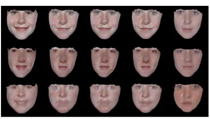
The results of ageing a face model using these methods is shown in figure 1.

Algorithm 5.2PLS ageing algorithm Train PLS model.

forFace modeliin the training setdo

Convert parameters of modelito Z-scores. ¯f=

f−ˆf

σ .

Calculate parameters in PLS space using gi =

(PTP)−1P¯fi, equation (13).

end for

Train Individualised Linear ageing model on PLS face modelsg.

Require: Input face model with parametersp

Convert parameterspto Z-scores.¯f=f−ˆf σ .

Convert p from PCA model space to PLS space.

g= (PT_P)−1_{P¯f, equation (13).}

Calculate residuals,r=¯f−gP.

Agegusing Individual Linear ageing model in PLS space.

Recover PCA parameters from PLS parameters.

¯f0_=g0_P.

Add residualsrto¯f0.

Convert from Z-scores to original model-space.

f0=¯f0σ+ˆf.

Figure 1: Examples of aged face images. Each row con-tains a different individual. The columns show, from left to right, the original mid-child face model for each indi-vidual, the mid-child face model aged to student age using the Prototyping method, the Individual Linear method and the PLS method. The right-most column shows the original face-model for the individual at student age.

Quantitative evaluation

The Mahalanobis distance between two sets of the face parameters has been used by (Lanitis et al., 2002; Lanitis et al., 2004; Scandrett et al., 2006) to measure the similarity between two faces in terms of the prob-ability that they are the same face.

d(a,b) =

s

∑

i

(ai−bi)2

σ2_i

(14)

wherea andb are two face models each composed

standard deviation of theith component of the PCA model.

In our case we can use this measure to determine the dissimilarity between an aged face and a known ground truth at the target ages. In order to determine the comparative effectiveness between different meth-ods of ageing we used a leave-one-out method. Fig-ure 2 shows the results of ageing using the proto-typing, individualized linear and PLS methods. We can clearly see that the ‘Individual Linear’ method gives an improvement in accuracy over the ‘Prototyp-ing’ method with a lower average error and the PLS method shows a marked improvement over both.

Table 2: Standard deviation weighted RMSE between shape and colour parameters of aged face model and a known ground-truth model for each individual in the data-set. With 93 subjects for each method.

Ageing Method RMSE Standard Deviation

Prototyping 8.86 1.84

Individual Linear 8.69 1.92

PLS 7.4 1.4

Perceptual evaluation

The Mahalanobis distance between two face models provides a quantitative description of the error be-tween the aged model and the known ground truth at the target age. However this measure may miss age-ing cues that human raters would be able to detect. We performed a series of tests with human raters to evaluate the ability of the methods to produce images of the required age.

Each user was shown a single image of a rendered face model at a time and asked to estimate the age of the face shown. The age is selected from a range between 5 and 30 to the nearest year. The stimuli are a selection mid-child faces aged to student age by the three-methods, prototyping, individualized linear and PLS, together with the rendered face-models of the individuals at the source and target age. Thus we have five groups for each individual in the face model data-set. The images are presented with the faces in a uniform pose, with uniform lighting conditions on a black background. Only the face is shown with no pe-ripheral details such as hair on display, as such ageing cues are limited to those in the face area. The images where presented on public website with users asked to estimate the age in years of the face shown. The website generated a significant amount of traffic, with an average of 105 age estimations per image, and just under 5000 for each ageing method being trialled.

Table 3 shows the mean perceived age in years

for the face models aged by the different methods as well as the mean ages of the rendered models of the original face models. Table 4 shows the mean age difference in years between the perceived age of the individual after the ageing method is applied and the target age the algorithm was attempting to recre-ate. We can see that all the methods succeed in age-ing the faces towards the target age, but vary in how much they age the face model. The worst method is the Individual Linear method ageing the faces to a mean of 16.801 and a mean difference of -3.8874, there is a statistically significant difference between the Individual Linear and the Prototyping methods ( p=0.026152, t=1.9408, dp=10180) using a one-tailed independent t-test and between the Individual Lin-ear and the PLS methods (p=0.017934, t=-2.3674, dp=9195). The PLS method also shows a statistically significant improvement over the Prototyping method (p=0.22495, t=-0.75562, dp=9145).

Table 3: Mean (µ) and standard deviation (σ) of the human rated ages for faces ages by each method

Ageing Method µ σ Count

Prototyping 17.048 6.7605 5090

Individual Linear 16.801 6.8449 5092

PLS 17.115 6.6780 4987

Student 17.026 5.9044 6205

Mid Child 12.762 6.0626 4678

Table 4: Mean (µ) and standard deviation (σ) of the error in years in human rated ages for faces ages by each method

Ageing Method µ σ Count

Prototyping -3.6614 6.1888 4596

Individual Linear -3.8674 6.1688 4646

PLS -3.5643 6.1098 4551

Student -3.3737 5.4273 5855

Mid Child 6.2135 6.0815 4678

7

CONCLUSIONS

Improved fitting techniques or a database of three-dimensional scans of the same person over several year, would improve the accuracy of these ageing methods. Other authors have used Quadratic and Cu-bic functions (Lanitis et al., 2002) in two-dimensions or non-linear Kernel methods such as Support Vec-tor Regression (Scherbaum et al., 2007) in three-dimensions, so and obvious extension is examine non-linear individualised ageing paths.

REFERENCES

Abdi, H. (2007). Partial least square regression (pls re-gression). InIn N.J. Salkind (Ed.): Encyclopedia of Measurement and Statistics., pages 740–744. Thou-sand Oaks (CA): Sage.

Baker, S. and Matthews, I. (2002). Lucas-kanade 20 years on: A unifying framework: Part 1. Technical Re-port CMU-RI-TR-02-16, Robotics Institute, Carnegie Mellon University, Pittsburgh, PA.

Blanz, V. and Vetter, T. (1999). A morphable model for the synthesis of 3d faces. InSIGGRAPH ’99: Pro-ceedings of the 26th annual conference on Computer graphics and interactive techniques, pages 187–194, New York, NY, USA. ACM Press/Addison-Wesley Publishing Co.

Gandhi, M. R., Levine, M. D., and G, M. R. N. (2004). A method for automatic synthesis of aged human facial images. Technical report, Masters thesis, McGill Uni-versity,2004. 1.

Hussein, H. K. (2002). Towards realistic facial modeling and re-rendering of human skin aging animation. In SMI ’02: Proceedings of the Shape Modeling Inter-national 2002 (SMI’02), page 205, Washington, DC, USA. IEEE Computer Society.

Hutton, T. J., Buxton, B. F., Hammond, P., and Potts, H. W. W. (2003). Estimating average growth trajecto-ries in shape-space using kernel smoothing. Medical Imaging, IEEE Transactions on, 22(6):747–753. Lanitis, A., Draganova, C., and Christodoulou, C. (2004).

Comparing different classifiers for automatic age esti-mation. IEEE Trans. Systems, Man and Cybernetics, 34(1):621–628.

Lanitis, A., Taylor, C. J., and Cootes, T. F. (2002). Toward automatic simulation of aging effects on face images. IEEE Trans. Pattern Anal. Mach. Intell., 24(4):442– 455.

Mark, L. and Todd, J. (1983). The perception of growth in three dimensions. Perception and Psychophysics, 33(2):193–196.

Park, U., Tong, Y., and Jain, A. K. (2008). Face recogni-tion with temporal invariance: A 3d aging model. In FGR06.

Pittenger, J. and Shaw, R. (1975). Aging faces as viscol-elastic events: Implications for a theory of nonrigid shape perception. J. Experimental Psychology: Hu-man Perception and PerforHu-mance, 1(4):374–382.

Pittenger, J., Shaw, R., and Mark, L. (1975). Perceptual information for the age level of faces as a higher or-der invariant of growth. J. Experimental Psychology: Human Perception and Performance, 5(3):478–493. Ramanathan, N. and Chellappa, R. (2006). Modeling age

progression in young faces. InIEEE Computer Vision and Pattern Recognition or CVPR, pages I: 387–394. Rowland, D. A. and Perrett, D. I. (1995). Manipulating fa-cial appearance through shape and color. IEEE Com-puter Graphics and Applications, 15(5):70–76. Scandrett, C. M., Solomon, C. J., and Gibson, S. J. (2006).

A person-specific, rigorous aging model of the human face.Pattern Recogn. Lett., 27(15):1776–1787. Scherbaum, K., Sunkel, M., Seidel, H.-P., and Blanz, V.

(2007). Prediction of individual non-linear aging tra-jectories of faces. In The European Association for Computer Graphics, 28th Annual Conference, EURO-GRAPHICS 2007, volume 26 ofComputer Graphics Forum, pages 285–294, Prague, Czech Republic. The European Association for Computer Graphics, Black-well.

Suo, J., Min, F., Zhu, S., Shan, S., and Chen, X. (2007). A multi-resolution dynamic model for face aging simu-lation. InIEEE Computer Vision and Pattern Recog-nition or CVPR, pages 1–8.

Tiddeman, B., Burt, M., and Perrett, D. I. (2001). Proto-typing and transforming facial textures for perception research.IEEE Computer Graphics and Applications, 21(5):42–50.

Tiddeman, B., Stirrat, M., and Perrett, D. I. (2005). To-wards realism in facial image transformation: Results of a wavelet mrf method. Comput. Graph. Forum, 24(3):449–456.

V. Bruce, M. Burton, T. D. (1989). Further experiment on the perception of growth in three dimensions. Percep-tion and Psychophysics, 46(6):528–536.

Wold, H. (1966). Estimation of principal components and related models by iterative least squares.Multivariate Analysis, pages 391–420.