The morphodynamics of a swash event on an erodible beach

Under consideration for publication in J. Fluid Mech.

The morphodynamics of a swash event on an

erodible beach

F. Zhu

†

and N. Dodd

1_{Department of Civil Engineering, University of Nottingham, Taikang Road, Ningbo, 315100,}

China

2

Infrastructure and Geomatics Division, Faculty of Engineering, University of Nottingham, Nottingham, NG7 2RD, England, UK

(Received ?; revised ?; accepted ?. - To be entered by editorial office)

A high accuracy numerical solution, coupling one-dimensional shallow water and bed-evolution equations, with, for the first time, a suspended sediment advection equation, thereby including bed- and / or suspended load, is used to examine two swash events on an initially plane, erodible beach: the event of Peregrine & Williams (2001), and that of a solitary wave approaching the beach. Equations are solved by the method of charac-teristics, and the numerical model is verified. Full coupling of suspended load to beach change for Peregrine & Williams (2001) yields only slightly altered swash flows, depend-ing on beach mobility and sediment response time; a series of similar final beach change patterns results for different beach mobilities. Suspended- and bed-load transport have distinct morphodynamical signatures. For the solitary wave a backwash bore is created (Hibberd & Peregrine 1979). This morphodynamical bore propagates offshore initially, and leads to the creation of a beach bed-step (Larson & Sunamura 1993), primarily due to bed-load transport. Its height is directly related to bed-load mobility, and also depends strongly on bed friction coefficient. The shock dynamics of this bed-step are explained and illustrated. Bed- and suspended-load mobilities are quantified using field data, and an attempt is made to relate predictions to measurements of single swash events on a natural beach. Average predicted bed change magnitudes across the swash are of the order of 2mm, with maximum bed changes up to about 10cm at the bed-step.

Key words:

1. Introduction

The swash zone is a very dynamic region in which the flow changes rapidly from sub-to supercritical, in which the beachface is repeatedly submerged and then dried, and in which there is also considerable sediment transported, as both bed and suspended load. The bed load maintains either continuous or intermittent contact with the bed (Masselink & Hughes 2003), and it responds to change in flow instantaneously, as therefore does the beach itself. The velocity and volumetric rate of bed-load sediment transport is difficult to quantify, and an empirical formula is usually used to describe this process. Suspended load is transported by the flow at the flow velocity, so the primary unknown is the concentration of sediment. Since it takes time for sediment to entrain into / settle out of the water column, both suspended sediment concentration in the water column and bed change caused by suspended load cannot in general adjust immediately to change

2 F. Zhu and N. Dodd

in flow (Pritchard & Hogg 2005). This means that the two modes of transport lead to a distinct, swash zone morphodynamics, which governs beach evolution in this region (also known as the beachface). Earlier papers (Pritchard & Hogg 2005; Kelly & Dodd 2010) have considered suspended load in isolation, or coupled bed load only with beach change. In this paper we present the first study to bring together bed- and suspended-load transport, and beach change, in a mathematical model, to describe and understand the dynamics of this region.

Sediment transport in the swash zone has been investigated in a number of field cam-paigns (e.g. Masselinket al.2008), but it is difficult to isolate physical processes in these energetic environments, and so analytical and numerical descriptions have been used to obtain understanding of erosive and depositional processes during single swash events. The beach change under one single swash event (that of Peregrine & Williams (2001), henceforth PW01) is examined by Pritchard & Hogg (2005) (henceforth PH05), by un-coupled simulations (i.e. simulations in which there is no feedback of bed change onto the flow within the swash event). Note that the mathematical solution embodied in the PW01 event was originally derived by Shen & Meyer (1963) for a wave approaching a beach; see also§3. Pritchard & Hogg (2005) examined only suspended load, with a series of sediment transport formulae. Results revealed the importance of settling lag (i.e. the time taken for sediment to settle out from suspension) in promoting deposition in the upper swash, as well as that of pre-suspended sediment (from the surf zone, or perhaps from the initial collapse of the bore at the base of the swash) in possibly dominating deposition. Without these effects the PW01 event was erosive for all sediment transport formulae examined.

Kelly & Dodd (2010), henceforth KD10, examined beach change under the same ini-tial PW01 event considering bed load only but fully coupling this to bed change. This approach is equivalent to assuming no settling lag and no pre-suspended sediment. This yielded net erosion throughout the swash, consistent with PH05, but with significantly less erosion than the equivalent uncoupled simulation. Zhu & Dodd (2013) subsequently examined a range of bed-load type formulae for PW01, as well as the influence of bed shear stress (as represented through a quadratic drag law description). All formulae yielded net erosion across the swash, although, generally, again reduced compared to equivalent uncoupled descriptions; bed shear stress was noted to reduce this erosion further, (due to decreased velocities) and, especially in the mid-swash, to promote depo-sition, particularly if the drag coefficient in the backwash were reduced, consistent with some observations, and the beach mobility reduced accordingly.

Guard & Baldock (2007) questioned the suitability of the PW01 event for describing most swash events, and presented a modified family of swash events, which allow for a more sustained flow up the beach. Pritchard (2009) examined the implications of this for erosion and deposition, noting that differences were quantitative rather than qualitative. Zhuet al.(2012) examined the beachface evolution under the swash event of Hibberd & Peregrine (1979), hereinafter HP79, using a similar, fully-coupled, bed load simulation to that in Kelly & Dodd (2010). This event yields large onshore momentum in the uprush (note that it is not the same as the uniform bore of Guard & Baldock (2007), because the bore originates on a constant depth region). Significantly, Zhuet al. (2012) observe the formation of a bed step (discontinuity in bed level), formed at the backwash bore (Hibberd & Peregrine 1979).

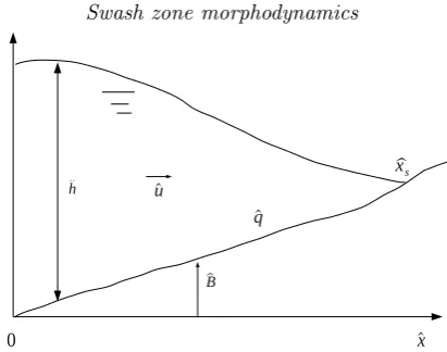
Figure 1.Schematic diagram for a general swash.

transport in the swash, and to see how they affect beach evolution during one swash event. In particular, we focus on the development of a beach bed-step, which is a com-mon feature of the swash (Larson & Sunamura 1993). To this end, we initially focus on the PW01 event, in order to allow comparison with earlier studies, and to examine the effects of bed- and suspended load. Thereafter, we focus on the bed-step formation, by examining a swash event due to a solitary wave, which is a commonly used, realis-tic model for a wave approaching the beach. We also use field measurements of beach change under single swash events on a natural beach to calibrate the unknown model parameters.

In the next section we present the model equations. We then examine the PW01 event in§3. In§4 we present the solitary wave event, and in§5 we estimate model parameters. Finally, we discuss our conclusions.

2. Model development

2.1. Governing equations

The nonlinear shallow water equations including bed shear stress described by a drag law (Soulsby 1997) are utilised to describe the flow in the swash zone

bh b

t+bubhbx+bhubbx= 0, (2.1)

b

u

b

t+ubbubx+gbhxb+gBbbx=−

cd|ub|ub

b

h , (2.2)

where bhrepresents water depth (m), u_b is a depth-averaged horizontal velocity (ms−1), b

B is the bed level (m),gis acceleration due to gravity (ms−2_{), andc}

d is a dimensionless drag coefficient. In figure 1 we illustrate the situation being considered.

The bed evolution (sediment conservation) equation including both bed- and suspended load is

b

B

b

t+ξqbbbx=ξ(Db−Eb), (2.3)

4 F. Zhu and N. Dodd

The governing equation for the transport of suspended sediment is

b

c

bt+ubbcbx=

1 b

h(Eb−Db), (2.4)

where_bcis volumetric concentration, andbh_bctherefore represents volume of sediment per unit area of sea-bed (m).

The Meyer-Peter M¨uller formula (see Yalin 1977; Soulsby 1997), which is commonly used in engineering problems, is employed

b

qb= ˆA

b

u2−_bu2_crb

ˆ

u2

0

3/2 |_bu|

b

u , (2.5)

where ˆu0 is a representative velocity scale, and ˆA a dimensional (m2s−1), empirically determined, representative bed load sediment transport rate.u_bcrbis the threshold velocity for sediment motion as bed load (ms−1_{). Note that ˆA=Auˆ}3

0, whereA is the equivalent dimensional constant of KD10.

We employ the entrainment model in Pritchard & Hogg (2003) and Pritchard & Hogg (2005), taking the entrainment rateEb =m_be

b

u2−ub

2 crs b u2 0

with m_be the parameter of sed-iment entrainment rate (ms−1_{) of suspended load, and}

b

ucrs the threshold velocity for sediment motion as suspended load (ms−1_{). Note that we set}

b

ucrb =ubcrs= 0 in all the simulations in the present work for simplicity. We expect that this simplification will not significantly affect beach morphodynamics except, perhaps, for shingle beaches, whereon permeability effects not considered here are also significant. See Appendix A.

The deposition rate of suspended load is (also following Pritchard & Hogg (2005)) b

D=w_bs_bcwithw_bsthe effective settling velocity of suspended sediment (ms−1). Therefore, (2.3) and (2.4) become

b

B

bt+ 3ξ

ˆ

A

ˆ

u3

0b

u2_bu

b

x=ξ

b

ws_bc−m_beb

u2 b u2 0 , (2.6) b c b

t+ubbcbx=

1 b

h

b

meb

u2

b

u2₀ −wbsbc

. (2.7)

2.2. Non-dimensionalization

The nondimensional variables are

x= xb

ˆ

h0

, t= bt

ˆ

h1₀/2g−1/2, h=

b

h

ˆ

h0

, u= ub

ˆ

u0

, B= Bb

ˆ

h0

, andc= bc

ˆ

c0

, (2.8)

where ˆh0is a length scale, ˆc0 is a reference concentration, and ˆu0= (gˆh0)1/2. Substituting (2.8) into the governing equations (2.1), (2.2), (2.6) and (2.7) gives

ht+uhx+hux= 0, (2.9)

ut+uux+hx+Bx=−

cd|u|u

h , (2.10)

Bt+

3ξAˆ

ˆ

h0(gˆh0)1/2

u2ux=

ξ

(gˆh0)1/2

b

wsˆc0c−m_beu2, (2.11)

ct+ucx=

1 (gˆh0)1/2ˆc0

1

h mbeu

2₋

b

wscˆ0c

. (2.12)

Let ˆc0= mbe b

ws,σ=

ξAˆ ˆ h0(gˆh0)1/2

,M =ξ mbe

(ghˆ0)1/2

and ˜E= wbs

(gˆh0)1/2

become

Bt+ 3σu2ux=M c−u2

, (2.13)

ct+ucx=

1

h

˜

E u2−c

. (2.14)

Note that here ˜E = Etanα, where E is the exchange rate parameter of Pritchard & Hogg (2005) and tanαis the beach slope. ˜E therefore governs the response time of the suspended sediment to changes in flow conditions.M represents bed mobility with regard to suspended load transport, andσthe equivalent quantity for bed load transport.

When sediment concentrationcis only determined by instantaneousu, it is denotedceq to represent suspended sediment concentration in an instantaneous equilibrium state (i.e. when there is neither erosion nor deposition); hereceq =u2. In (2.14), when ˜E/h→ ∞, the adjustment ofctoceq becomes immediate. Note thatceq=ceq(x, t).

The vector form of these four non-dimensional governing equations is

− →

Ut+A(

− →

U)−→Ux=

− →

S (2.15)

with

− →

U =



  

h u B c



  

,A(−→U) =



  

u h 0 0

1 u 1 0

0 3σu2 _{0 0}

0 0 0 u



  

,

− →

S =



  

0

−cd|u|u

h

M c−u2

1 hE u˜

2_−c 

  

.

The eigenvalues ofAare the roots of the polynomial equation

(λ−u)(λ3−2uλ2+ (u2−3σu2−h)λ+ 3σu3) = 0. (2.16) The polynomial equation (2.16) has four roots, one of which λ4 ≡u, corresponding to the transport of suspended load. The other three roots of (2.16) are denotedλ1,λ2 and

λ3 such that λ1 6 λ3 6 λ2. Note that if σ 6= 0 and h 6= 0, when u > 0, we have

λ1< λ3< λ4< λ2; whenu <0,λ1< λ4< λ3< λ2. Also,λ1<0, andλ2>0 as long as

σ6= 0. For the solution ofλ1,λ2 andλ3 we refer to Kelly & Dodd (2009, 2010).

Figure 2 illustrates theλ1,2,3 characteristics variation with Froude number whenσ= 0.01. Note that individual characteristics, λ1,2,3, can “behave” as hydro- or morphody-namic characteristics, depending on Froude number. It can be seen that there are sudden changes in these roles at critical flow conditions. From simple wave theory (Jeffrey 1976), a shock exists when the characteristics of the same family intersect, and it is aλi shock if it is theλi characteristics that intersect.

2.3. Numerical method

The specified time interval method of characteristics (STI MOC) (Kelly & Dodd 2009, 2010), which can resolve shocks very accurately, is used to solve (2.9), (2.10), (2.13) and (2.14) simultaneously. As theλ1,2,3characteristic fields associated with (2.9), (2.10) and (2.13) are genuinely nonlinear, and theλ4associated with (2.14) is genuinely linear, (2.9), (2.10) and (2.13) are combined to get total derivatives (i.e. the characteristic form) ofh,

6 F. Zhu and N. Dodd

−2 −1 0 1 2

−4 −2 0 2 4

F

λ

/

√

h

λ 1

λ 2

λ 3

Figure 2.Variation of dimensionless wave velocities with Froude number (Fr=u/√h) for system with bed load transportq=u3 (σ= 0.01).

<(k)=λk

du

dt +

λk

λk−u

dh

dt +

dB

dt =−λk

cd|u|u

h +M c−u

2

along dx

dt =λk, k= 1,2,3,

(2.17) and (2.14) is written as the total derivative ofcwith respect to time

dc

dt =

1

h

˜

E u2−c

, along dx

dt =λ4=u. (2.18)

These four equations of (2.17) and (2.18) are solved numerically to geth,u, B andcin the combined load system.

2.3.1. Initial conditions

Initial conditions are given for each case examined, but one general point concerns initial values for c and B. Any pre-suspended sediment must be included as an initial condition: c =c(x,0). Note that, depending on whether c(x,0) < or > ceq, the initial

B will immediately erode or accrete due to suspended load. Here, c(x,0) = ceq in all simulations unless otherwise specified.

2.3.2. Seaward boundary condition

The seaward boundary is chosen so as to be far enough away from the shore that h

and uat that point are uninfluenced by any wave reflected from the shore throughout the computation time. Consequently, the seaward boundary is chosen atx=−150. Note that for both events examined there is therefore a region of uniform flow adjacent to this boundary, in which the flow can be specified analytically. Other dependent variables at the seaward boundary may be extrapolated from values at neighbouring points. Thus, we haveh(−150, t) =hof f andu(−150, t) =uof f−tanαof ft, where tanαof f is the bed slope atx=−150, and B andc are extrapolated from neighbouring points. Note that this boundary is therefore not specified based on incoming and outgoing characteristics, although characteristics at this location can straightforwardly be calculated.

2.3.3. Wet-dry boundary treatment

At the tip (shoreline),x=xs(t),h(xs) = 0, andc(xs) =ceq =u2s. For the solution of

2.4. Shock conditions

For derivations of shock conditions for mass and momentum conservation we refer to Kelly & Dodd (2010); Zhuet al.(2012); the shock conditions are

hRuR−hLuL−(hR−hL)W = 0, (2.19)

W(hRuR−hLuL)−

hRu2R+

h2

R 2 −hLu

2 L−

h2

L 2

−1

2(BR−BL)(hR+hL) = 0, (2.20) whereLandR represent variables on the left and right side of a shock, andW is shock velocity.

For the bed evolution, the change of bed level in the fixed domain [x1,x2] is balanced by the net sediment flux into (out of) that domain, and also the net sediment settlement onto (or entrainment from) it, thus

d dt

Z x2

x1

Bdx+ [σu3]x2

x1=

Z x2

x1

M c−u2dx. (2.21)

Here it is also assumed that a shock located at ζ(t) lies between x1 and x2, i.e., x1 <

ζ < x2. In the limitx1→ζ andx2→ζ, (2.21) becomes

−W[B]x2

x1+ [σu

3_]x2

x1 = 0. (2.22)

It is found that suspended load has no contribution to the shock condition for the bed evolution.

The suspended sediment in the water column in the domain [x1,x2] is balanced by the net suspended sediment flux inflow acrossx1 andx2sections and the entrainment from (settlement onto) the bed, thus

d dt

Rx2

x1(hc)dx+ [huc]

x2

x1=

Rx2

x1 M u

2_−c

dx

⇒ [−hcW +hcu]x2

x1 = 0. (2.23)

(2.22) and (2.23) can then be written as

(BR−BL)W −σ(u3R−u 3

L) = 0, (2.24)

hRcR(uR−W)−hLcL(uL−W) = 0. (2.25) Note that the shock condition of the bed evolution (2.24) in the combined load system is identical to that without suspended load in Kelly & Dodd (2010).

For aλ1,2,3 shock, if hL 6= 0, hR 6= 0, uL 6=W and uR 6=W, from (2.19), the shock condition for the transport of suspended load (2.25) is simplified as

cR−cL= 0. (2.26)

This implies that the sediment concentration across aλ1,2,3 shock is continuous, and it is determined by the genuinely linear characteristic field associated with the transport of suspended sediment.

For aλ4 shock, which is a contact wave, we have hL =hR, uL =uR, BL =BR and

cL6=cR.

For the shock fitting method, we refer the reader to Kelly & Dodd (2010), who have described the technique in great detail.

2.5. Model testing

8 F. Zhu and N. Dodd

−50 −40 −30 −20 −10 0 10 0

0.2 0.4 0.6 0.8 1 1.2 1.4 1.6

x

B

,B

+

h

Hw

B h

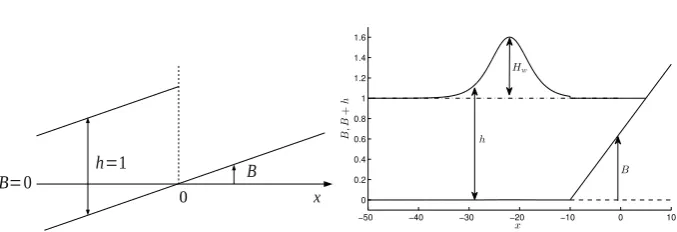
Figure 3.Initial conditions for PW01 (left) and solitary wave swash (right).

B, we compare with PH05 results, which are for suspended load, on a nearly fixed bed. Testing of the bed-load-only model is presented in Zhuet al. (2012).

3. PW01 swash event

In this section, we aim to elucidate the effects of bed- and suspended load as represented byσ,M and ˜Eby modelling a swash event morphodynamically. We examine the PW01 event here. As noted earlier, although this event is not considered representative of many swash events (Guard & Baldock 2007), in terms of sediment transport it can be considered qualitatively similar (Pritchard 2009). Furthermore, using it allows us to verify against earlier work (see Appendix B), and also to examine a swash event in which no significant interior shock formation takes place. Therefore, we consider a swash event with the same initial conditions as the PW01 swash, which then evolves morphodynamically; we refer to it hereafter as the PW01 event. Note that this shoreline motion was originally derived by Shen & Meyer (1963). We refer to it here as the PW01 event because these authors, who extended the analytical solution for the shoreline motion to whole swash and examined overtopping due to this event, provided it in a more accessible form, and made the connection between the same swash motion as the result of a dam-break problem, which interpretation we make use of as our initial condition.

The initial conditions of the PW01 swash are described by a dam-break problem over an erodible beach of initially uniform slope B = tanαof fx (Kelly & Dodd 2010) (see figure 3). The dam is situated atx= 0 with still water on the seaward side and none on the shoreward side. The water depth behind the dam ish(x <0, t= 0) = 1. The dam is assumed to collapse att= 0, and the flow is dominated by gravity.

3.1. Suspended load

A suspended-load-only simulation is achieved by setting the bed mobility parameter for bed loadσ= 0 in the combined load model.

The final bed changes after one swash event for various M values (σ= 0) with and without pre-suspended sediment are shown in figure 4 (a) and (b). The effect of varying

M can be seen. For σ= 0, (2.13) shows the linear relationship between bed change and suspended load mobility M: as long as the flow remains largely unaffected by the bed change ( ˜E is constant) ,c will remain similarly unaffected by varying M, and a change in M results in a similar but amplified pattern of erosion and deposition, i.e. ∆B ∝M

pre-0 5 10 15 20 −0.1

−0.05 0

x( ˜E= 0.001)

∆

B

(a)

M= 1×10−4

M= 5×10−4

M= 1×10−3

M= 5×10−3

0 5 10 15 20

0 0.02

0.04 _(b)

x( ˜E= 0.001)

∆

B

0 5 10 15 20

−25 −20 −15 −10 −5 0 5

x( ˜E= 0.001)

∆

B

/M

(c)

M= 1×10−4

M= 5×10−4

M= 1×10−3

M= 5×10−3

0 5 10 15 20

0 2 4 6 8 10

(d)

x( ˜E= 0.001)

∆

B

/M

0 5 10 15 20

−2.5 −2 −1.5 −1 −0.5 0

0.5x 10

−3

x(M= 1×10−4)

∆

B

(e)

˜

E= 0.001 ˜

E= 0.005 ˜

E= 0.01 ˜

E= 0.03

0 5 10 15 20

0 2 4 6 8

10x 10

−4

(f)

x(M= 1×10−4)

∆

B

Figure 4. Upper panels: Bed change after one PW01 swash event for various M values ( ˜E = 0.001), for (a) only locally entrained sediment; and (b) with both locally- and pre– suspended sediment (c0 = 1). Middle panels: Bed changes for the same simulations shown,

respectively, in (a) and (b), normalised by M. Bottom panels: Bed changes after one PW01 swash event for various ˜E values (M = 1×10−4_{), for (e) only locally entrained sediment; and}

(f) with both locally- and pre-suspended sediment (c0= 1).

suspended sediment. Only forM = 0.005 do we see a noticeable change in the resulting beach change profile (see figure 4 (c) and (d)).

The effect of ˜Eon the net sediment flux was discussed in depth by Pritchard & Hogg (2005). In figure 4(e) and (f), we show a variety of resulting profiles for different ˜E, now with a fully mobile bed. As ˜Eincreases there is less net movement overall. This is due to the erosion / deposition term in (2.13) (c−u2) being near zero for larger ˜E (consistent with PH05) for most of the swash event, because c ≈ ceq (because of the more rapid adjustment as ˜E increases). Therefore, overall beach change is reduced (for fixed M) (See also figure 21 for verification against PH05 in terms of net fluxes). This is illustrated in figure 5.

Additionally, when pre-suspended sediment is present (figure 4 (f)) net change increas-ingly favours deposition at the base of the swash. This is again consistent with PH05, and stems from the fast response time for larger ˜E causing initially entrained sediment to be immediately deposited (in the lower swash).

10 F. Zhu and N. Dodd

0 5 10 15 20

0 5 10 15 20 25 30 35 40

x

t

−0.5 −1

−0.1 −0.05 −0.01 0 0.01 0 −0.01

−0.05 −0.1 −0.5

−1

0.05

0.1 _0.2 0

−0.01 −0.05 −0.1

(a)

0 5 10 15 20

0 5 10 15 20 25 30 35 40

x

t

−0.01 −0.05

0

0.01

0.05

0.1 −0.1

−0.1

−0.05

0.01 0.05

−0.1

−0.5

−1

−0.01 −0.05

(b)

Figure 5.Contour plots forc−u2 for simulations in figure 4. (a): ˜E= 0.001, and (b):

˜

E= 0.03.

flux across the swash zone caused by locally entrained sediment, which essentially is a measure of the total amount of deposition in the swash zone. Moreover, the work of Pritchard & Hogg (2005) (see figure 11(a) and (c) of PH05) has further indicated a peak value in the proportion of deposited to eroded sediment flux / volume. For ˜E→ ∞, this ratio→0, as expected.

3.2. Suspended and bed load

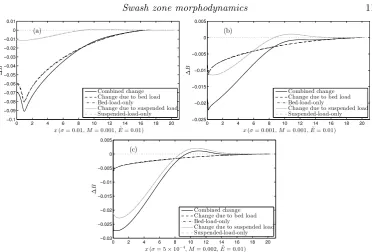
If we include both suspended and bed load we can now examine their effects on the beach during this event. The final bed changes in three combined load simulations are shown in figure 6, and correspond to beaches in which either bed- or suspended load are dominant, or about equal. Also shown are the bed changes caused by the equivalent bed-load only and suspended-load only simulations, and that due only to those same components of the combined load simulation. Note that, for the parameters chosen here, each mode of sediment transport has little effect on the other, and each has a distinct morphodynamical signature, and these are consistent with the results of Pritchard & Hogg (2005) and Kelly & Dodd (2010).

4. Swash event with shock formation

In this section, a swash event that involves shock formation in the swash zone is sim-ulated to examine the effect of more representative swash event on an erodible beach, and in particular, to study the bed step development associated with the backwash bore (Hibberd & Peregrine 1979; Zhuet al.2012). Initially we exclude bed shear stress, and focus on the shallow water dynamics and backwash bore and bed-step developments, and consider what happens when the shoreline encounters this feature. Thereafter we intro-duce bed shear stress and consider the shock dynamics that contribute to the bed step development. A swash event driven by a solitary wave is examined. The event represents a simplified but physically appropriate model of a surface gravity wave encountering a beach.

4.1. Solitary wave event

0 2 4 6 8 10 12 14 16 18 20 −0.1

−0.09 −0.08 −0.07 −0.06 −0.05 −0.04 −0.03 −0.02 −0.01 0 0.01

x(σ= 0.01, M= 0.001,E˜= 0.01)

∆

B

(a)

Combined change Change due to bed load Bed-load-only

Change due to suspended load Suspended-load-only

0 2 4 6 8 10 12 14 16 18 20

−0.025 −0.02 −0.015 −0.01 −0.005 0 0.005

x(σ= 0.001, M= 0.001,E˜= 0.01)

∆

B

(b)

Combined change Change due to bed load Bed-load-only

Change due to suspended load Suspended-load-only

0 2 4 6 8 10 12 14 16 18 20 −0.03

−0.025 −0.02 −0.015 −0.01 −0.005 0 0.005

x(σ= 5×10−4_{, M= 0.002,}E˜= 0.01)

∆

B

(c)

Combined change Change due to bed load Bed-load-only

Change due to suspended load Suspended-load-only

Figure 6.Bed changes in the combined load simulations and comparisons with bed-load-only and suspended-load-only simulations after one single PW01 swash. (a) Bed-load dominance; (b) bed- and suspended-load approximate parity; and (c) suspended-load dominance.

surface profile for a solitary wave given by Mei (1990), with h(x < −10, t = 0) = 1 +Hwsech2

0.33Hw

4h3 st

1/2

(x+ 22)

. The water velocity is then determined by the hydrodynamic Riemann invariant along the backward characteristic:u(x <−10, t= 0) = 2(ph(x, t= 0)−1). The bed level is adjusted to the water flow withB(x <−10, t= 0) =

σ√u(x,t)3

h(x,t). However, the water flow is assumed not to be affected by the bed change at the initial time. Across the domain,c(x, t= 0) =ceq(x, t= 0) =u2(x, t= 0) is assumed.

4.2. Simulation without bed shear stress

The flow structure as a solitary wave travels shorewards over an erodible beach (σ= 0.01,

M = 0.001 and ˜E = 0.01) simulated by the combined load model is shown in figure 7. When the solitary wave travels shorewards, it breaks and forms a shock (bore) travelling to the shore. The shock then collapses at the initial shoreline position (x= 5), and then the water climbs up the dry beach. The water velocity reaches its maximum when the shock collapses, and then decreases when the flow climbs up the dry beach. The flow (in the region x >5) is similar to that in the PW01 swash (cf. figure 7(a) and figure 22). This is because the wave breaks at the base of the swash with little water momentum behind it, similar to the PW01 event (see Guard & Baldock 2007).

12 F. Zhu and N. Dodd (a) x t 0.001 0.01 0.05 0.1 0.15 0.2 0.25 0.3 0.35 0.4 0.5 0.6 0.7 0.8 0.9 1 1.2 1.4

10.9 0.80.7 0.6

−10 0 10 20 30 40

0 10 20 30 40 50 60 70 80 (b) x t −2.2 −2 −1.8 −1.6 −1.4 −1.2 −1 −0.8 −0.6 −0.4 −0.2 0 0.2 0.4 0.6_0.8 1 1.2 1.4 −0.2 −0.2 −0.4 0 0.2 0.4 0.6

−10 0 10 20 30 40

0 10 20 30 40 50 60 70 80 (c) x t 0 −0.005 −0.01 −0.02 −0.03 −0.04 −0.05 −0.06 −0.07 −0.08 −0.09 −0.1 −0.06 −0.07 −0.05 −0.04 −0.03 −0.02 −0.01 −0.005 0 0.005 0.01 0.02 0.005 0

−0.005 −0.01 −0.02 −0.03 0 0.005 0.5 0.20.1 0.05 −0.01 0.02 −0.1 0

−10 0 10 20 30 40

0 10 20 30 40 50 60 70 80 (d) x t 0.01 0 0.05 0.1 0.10.05 0.01 0.5 1 2 1.5 0.5 1 1.5 2 2.5 3 3.5 4 4.5 5

−10 0 10 20 30 40

0 10 20 30 40 50 60 70 80 (e) x t Deposition Erosion Erosion Deposition

−100 0 10 20 30 40

10 20 30 40 50 60 70 80

Figure 7.Contour plots for the combined load solitary wave swash simulation over an erodible beach (σ= 0.01,M = 0.001 and ˜E= 0.01). (a):h; (b):u; (c): ∆B; (d):c; (e): instantaneous deposition / erosion distribution due to suspended load. The thick black dashed line in (e) represents the backwash bore path.

Note that at the shorelinec=ceq=u2s, and at the maximum inundation is 0. This is because as the tip is approached E_h˜ → ∞, so that there is an instantaneous adjustment ofc toceq. For the whole backwash (forx >5), c < ceq, and sediment is entrained into the water column and moved seawards, and the beach eroded; see figure 7(d), (e).

Bed load transport results in erosion everywhere (not shown) (becauseq_bx>0 every-where), except at the shoreline, where there is instantaneous increase (decrease) in B

bed-load-only simulations for the HP79 swash event (Zhuet al.2012). The development of a backwash bore can be seen in figure 7 (a) and (b). The strength gradually increases, with increasing differences in h, u and B on the two sides of the shock, and therefore leads to the development of a bed step coincident with the bore; this shock moves offshore and gradually slows. The shoreline eventually catches up with this shock, leading to a fully developed bed step at the base of a dry beach; see§4.3.

Across the shockuis discontinuous, andccontinuous ((2.19), (2.20) and (2.26)), which results in entrainment and erosion (deposition and accretion) on the shoreward (seaward) side of the bed-step as (from) suspended load (see (2.13)). This continues until sediment concentrationcon the shoreward side exceedsceq, at which point the boundary between suspended load erosion and accretion departs from the shock path (figure 7(e)).

It is the bed-load that is most closely linked with the bed-step development, however, as this responds instantly to all flow changes in the vicinity of the shock. Across the shock the massively different bed-load transport rates (qb) result in accretion immediately seaward of the shock, and development and offshore propagation of the bed-step. Note, however, that shoreward of the shock there is also local accretion due to convergence of bed-load transport. This is caused by corresponding, initially small gradients in u (figure 7(b)) shoreward of the shock, which instantly affectqb (unlikeqs), leading to local deposition. Thus, the bed-step both advances seawards, and grows in height.

Note that although suspended load can affect a moving bed discontinuity through changed erosion / accretion rates across the shock, and by modifying the beach profile generally, the bed-step height and velocity are directly linked to bed load transport (as long asW 6= 0; see (2.24)).

4.3. Analysis of when the shoreline catches up with the backwash bore

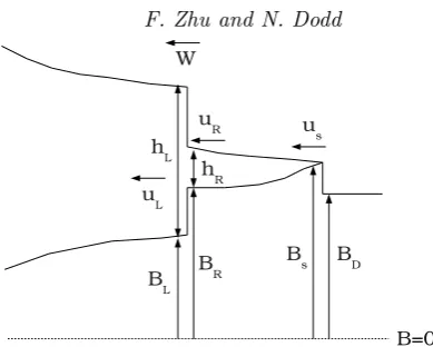
In the simulation without bed shear stress, the shoreline eventually catches up with the backwash bore. As there is a sediment bore at the shoreline, this is a shock-shock collision. In this situation there are three regions, with the rightmost being dry, and in which the right shock (the shoreline) is wet-dry, and the left (backwash bore / bed-step) a wet-wet shock: see figure 8.

As the two shocks come closer, the middle region gradually vanishes, and in the limiting case this region converges to one point, such that values of dependent variables on the left and right extremities of this region become equal. Therefore, at the moment of the two shocks colliding, the middle region is assumed to disappear and the flow has only one newly formed discontinuity; however, the shock conditions are then usually not satisfied at this new discontinuity, which is therefore not stable and collapses, with the resulting states found by solution of a local Riemann problem. This is not pursued here.

As the middle region width→0,hR→0 anduR → dx_dts =us. As the numerical code cannot proceed when the two shocks are very close, the numerical solution is only an approximation for the case of zero middle region width. The analytical solution for the backwash bore (Appendix E), of which one side is a nearly dry bed but with water of finite velocity, can be utilised to obtain the limit flow structure right before the shock collision.

From Appendix E, when the shoreline approaches the backwash bore

BR−BL →hL−hR→hL. (4.1)

Across the sediment bore at the shoreline we haveBD=BR−σu2s. Thus, as the shoreline approaches the bed step:

14 F. Zhu and N. Dodd

Figure 8.Schematic diagram for two shock collision.

Therefore, the resulting (post-collision, unstable) bed step height will be slightly lower than the water depth on the seaward sidehL. The water on the seaward side may overtop the bed step, depending on the velocity and also bed mobility.

4.4. The inclusion of bed shear stress

The contour plots for the solitary wave simulation with bed shear stress (σ = 0.01,

M = 0.001, ˜E = 0.01 and cd = 0.01) are shown in figure 9. Note that the shoreline does not recede in the backwash (Antuonoet al. 2012; Zhu & Dodd 2013), because of bed friction, and the swash zone is always wet once wetted. Note that the corresponding swash period is much longer than forcd= 0. The flow structure in the uprush is similar to that in the simulation without bed shear stress, with an overall deeper flow and smaller velocity. However, bed shear stress greatly reduces the seaward velocity of the backwash flow, and the backwash duration exceeds that of the uprush. The bed shear stress also modifies the flow structure in the backwash, and more shocks are formed in the backwash. The shock paths (including inception and termination points) are illustrated in figure 9 (a)-(c). Note that the first shock to form (aλ1shock) does so at aboutt= 23.5. It quickly propagates offshore, and has no influence on the subsequent bed-step development, so we ignore it hereafter. Note the values ofcin figure 9(d) are considerably reduced compared to those in figure 7(d), especially during the backwash, consistent with reduced backwash velocities.

In the backwash, a bore (λ3shock) develops (the backwash bore), which initially trav-els seawards (see figure 9). This is a robust feature of the backwash (see also figure 7(a)). Att ≈61.4, another, weaker λ3 shock collides with the backwash bore. Here, we treat the shock collision by neglecting the weaker shock when it is in close proximity to the backwash bore. This approach shows good agreement with the idealised Riemann solu-tion. The collision increases the backwash bore (λ3) shock strength slightly; see figure 10. Thereafter, the backwash bore slows, and decreases in strength (see figure 10).

Att≈67.7, aλ2shock develops on the shoreward side of the backwash bore / bed-step, the strength of which rapidly increases (see figure 10), and which propagates shoreward, as the flow in the later backwash diminishes. Thereafter it diminishes and slows, in effect re-establishing a “shoreline” boundary between the sea and water still draining back. Note that, as with all morphodynamical shocks, thisλ2 shock is accompanied by a bed discontinuity, which travels with the shock, but which is much smaller than the bed-step associated with the originalλ3backwash bore / bed-step, see figure 10.

(a) x t 0.001 0.01 0.05 0.1 0.15 0.2 0.25 0.3 0.35 0.5 0.6 0.7 0.8 0.9 1 1.2 0.2 0.150.1 0.05 0.3 0.35 0.4 0.5 0.6 0.7 0.8 0.4 0.4

−100 −5 0 5 10 15 20 25

10 20 30 40 50 60 70 80 90 100 (b) x t −0.1 −0.05 −0.2 −0.4 0 −0.05 −0.1

−0.2 −0.7 −0.6 0.1 0.05 0 0.05 −0.4 −0.2 −0.1 −0.05 0 0.2 0.4 0.6 0.8 0.6 0.4 0.2 −0.2 0.1 0.05 −0.05 0

−100 −5 0 5 10 15 20 25

10 20 30 40 50 60 70 80 90 100 (c) x t 0 0 0.005 −0.01 −0.005 0 0.01 −0.01 −0.005 −0.01 0.005 0 0.03 0.01 −0.005 0.005 0.05 −0.005

−100 −5 0 5 10 15 20 25

10 20 30 40 50 60 70 80 90 100 (d) x t 0.01 0.05 0.1 0.2 0.1 0.05 0.01 0.2 0.3 0.3 0.01 0.2

−10 −5 0 5 10 15 20 25

0 10 20 30 40 50 60 70 80 90 100

Figure 9.Contour plots for solitary wave simulations with bed shear stress over an erodible beach (σ= 0.01,M = 0.001, ˜E= 0.01 andcd= 0.01). (a)h; (b)u; (c) ∆B; and (d):c. In (a), (b) and (c) we show the shock paths of theλ3 andλ2 shocks, with their points of inception and

termination. Dotted line:λ1 shock; dot-dashed line: firstλ3 (weak) shock; dashed line: second

λ3 shock (backwash bore); solid line:λ2 shock.

16 F. Zhu and N. Dodd

1 2 3 4 5 6

0 0.1 0.2 0.3 0.4

Shock position

x

λ

L

−

λ

R

(a)

λ

3 shock

λ

2 shock

1 2 3 4 5 6

−0.12 −0.1 −0.08 −0.06 −0.04 −0.02 0

0.02

(b)

Shock position

x

B

L

−

B

R

0 0.1 0.2 0.3

−0.12 −0.1 −0.08 −0.06 −0.04 −0.02 0

0.02

(c)

λ

₋

λ

B

−

B

−2 −1.5 −1 −0.5 0 0.5

−3 −2.5 −2 −1.5 −1 −0.5 0

(d)

F

F

R

Figure 10.Shock strength and Froude number forλ2 andλ3 shocks in the backwash.

represents the inception of a shock.

reason (note that the definition of shock strength here is the jump in characteristic slope across the shock). See also figure 10(a) and (d). Note that the weakλ3 shock does not pass through critical conditions.

Finally, in figure 11 we show the characteristic fields associated with the shock dynam-ics described above. The characteristic convergence and shock formation can clearly be seen.

4.5. Final beach change and bed-step development

−100 −5 0 5 10 15 20 25 20

40 60 80 100

x

t

0 1 2 3 4 5 6

40 50 60 70 80 90 100

x

t

Figure 11.Characteristics diagram for the solitary wave simulation with bed shear stress: (a) for the whole domain; (b) for the vicinity of the reversing shock. Grey solid lines:λ1characteristics;

black dashed line:λ2 characteristics; and black solid lines:λ3 characteristics. The thick black

solid, dashed, dash-dot and dotted lines represent the paths of the backwash bore,λ2 shock,λ3

shock andλ1 shock, respectively.

−10 0 10 20 30 40 50

−0.2 0 0.2 0.4 0.6 0.8

x

∆

B

σ= 1_×10−3, M= 1_×10−4

σ= 1_×10−3, M= 1_×10−3

σ= 0.01, M= 1_×10−4

σ= 0.01, M= 1_×10−3

Figure 12.Final beach changes for solitary wave simulations without bed shear stress for two different values ofσandM.

prominence of the step is dictated by σ (figure 13). Note also the increased erosion shoreward of the step for largerM (figure 12).

To examine importance of the swash event on the bed-step generation, the final water surface profiles and bed changes for both the present solitary wave simulation and those for the HP79 swash (see Zhu et al.2012) (both forcd = 0) are illustrated in figure 14. Note that both events have the same wave height, but that the HP79 event is essentially an adjustment in water level, so that the backwash (and therefore backwash velocities) is (are) much reduced compared to the uprush. Note also that the bed-steps for the solitary wave case including friction (figure 15), in which backwash velocities are significantly reduced and no longer dependent solely on maximum run-up, are consistent with those for the frictionless HP79 case. The bed step heights in both swashes are close to but slightly smaller than the water depths due to the sediment bore at the tip, consistent with the analysis in§4.3.

18 F. Zhu and N. Dodd

0 0.2 0.4 0.6 0.8 1

x 10−3 0.3

0.4 0.5 0.6 0.7 0.8 0.9 1

M

B

ed

st

ep

h

ei

g

h

t

(a) σ=1×10−5

σ=0.001

σ=0.01

−6 −5 −4 −3 −2 −1 0

−0.2 0 0.2 0.4 0.6 0.8

x

∆

B

(b) M=0

M=0.0005 M=0.002 M=0.005

Figure 13.Bed step heights and final beach changes for solitary wave simulations without

bed shear stress for differentσandM values ( ˜E= 0.01).σ= 0.01 in (b).

−200 −10 0 10 20 30 40 50

0.5 1 1.5 2 2.5 3 3.5 4

(a)

Bed step due to a uniform bore →

Bed step due to a solitary wave

↓ ↑

←

←

u

u

SWL

x

B

,

B

+

h

−10 0 10 20 30 40 50

−0.2 −0.1 0 0.1 0.2 0.3 0.4 0.5

0.6 (b)

x

∆

B

Figure 14.Beach profiles (a) and changes (b) under a solitary wave (black) and the HP79 swash (grey) withσ= 0.01,M = 0.001 and ˜E= 0.01 (cd= 0).

−10 −5 0 5 10 15 20 25

−0.2 0 0.2 0.4 0.6

x

∆

B

cd= 0

cd= 0.005

cd= 0.01

cd= 0.02

Figure 15.Final beach changes for solitary wave simulations with bed shear stress for various

cdvalues (σ= 0.01,M= 0.001 and ˜E= 0.01).

10−3 10−2 0.2

0.4 0.6 0.8 1 1.2 1.4 1.6 1.8

2x 10 −3

˜

E

M

110

100

90

80

70

60

50

40

30

20

10

5

Figure 16.Contour plot of dimensional suspended-load fluxρsˆh20ˆc0Qen,up(x= 13) as a function

of ˜EandM after the uprush of one single solitary wave swash withcd= 0.01 (Units kg/m).

5. Estimation of

M

and

σ

from field experiments

Finally, we note that it is difficult to evaluateMfor real beaches ( ˜Emay more straight-forwardly be evaluated from settling velocities). In an attempt to do this we present figure 16, in which we show a contour plot of net onshore flux of suspended sediment entrained in the uprush only, at a location in the mid-swash (x= 13) of the solitary wave swash event (Qen,up(13); see Appendix C for the definition of net fluxQ) with bed shear stress (cd= 0.01) as a function of M and ˜E. This position is roughly equivalent to that of sediment traps in Masselink & Hughes (1998) and Hugheset al.(1997). Both studies, which were for grain sizes and beach slopes of, respectively, 0.5mm and 0.14, and 0.3mm and 0.12, yielded representative, average onshore fluxes in moderate wave conditions of

∼30kg/m over one swash uprush. Thus, a grain size of 0.4mm (ws≈0.05m/s⇒E˜≈0.02 if ˆh0= 1m) corresponds to a value ofM ≈0.001.

As with determining M, determiningσ is an uncertain process, but its effect can be quantified similarly to that ofM in variation of net uprush bed-load flux

Qb(x) =

Z tde

tin

σu3dt (5.1)

in the mid-swash (wheretin(tde) is the time of inundation (denudation) ): see figure 17. A net flux of 30kg/m due to bed load thus corresponds toσ≈0.01. Further, note that figure 6 implies that assuming that suspended- and bed-load transport do not significantly affect each other, as done in figure 16 and 17, is reasonable.

20 F. Zhu and N. Dodd

0 0.005 0.01 0.015 0.02 0.025 0.03 0.035 0.04 0.045 0

20 40 60 80 100 120 140

σ

ρ

ˆ

h

2 0

Q

b,

u

p

/

ξ

(k

g

/

m

)

Figure 17.Variation of dimensional bed-load fluxρsˆh20Qb,up/ξ(x= 13) as a function ofσ

after the uprush of one single solitary wave swash withcd= 0.01 (Units kg/m).

to examine how assuming different proportions of each mode within this representative event affects the resulting concentrations and the eventual bed-step geometry.

5.1. Proportions of bed- and suspended load.

We use figure 16 and figure 17 to allocate a proportion of the nominal 30kg/m to each mode. These allocations are summarised in Table 1, and correspond roughly to a scenario in which bed and suspended load are both significant (Test 1), which therefore comprises our best estimate of reality; and two further ones in which bed (Test 2) or suspended (Test 3) load dominates. Finally, in Test 4, we consider a case in which pre-suspended load dominates. Therefore, for Test 4, we reduce local bed and suspended loadQvalues (and thereforeM and σ) and then impose c at the time of bore collapse at the shore:

t =tc. This is to reproduce the large local concentrations that might be expected due to bore turbulence, which is not present in the mathematical model. The approach here is to impose c(x, t = 0) =ceq(x,0) and c(x, tc) =nceq(x, tc), and to determinen such that the net total, mid-swash onshore flux is 30kg/m. This results inn= 1.8. Note that pre-suspended load exists in Tests 1-3 too, but only at equilibrium values (at t = 0). Therefore, much of the sediment initially present falls out of suspension prior to bore collapse: see§4.1. The volume of sand in each bed-step ( ˆV) is also presented in Table 1, and is calculated from the base on the left side ∆B= ∆BL to the position on the right side such that ∆BR= ∆BL, see figure 19(b).

5.2. Concentrations and final bed profiles

The contour plots of ˆc for four test cases are shown in figure 18. The suspended load dominant case Test 3 has the largest concentration with the maximum of∼0.01. In the uprush the effect of the pre-suspended sediment can still be seen but not in the backwash (figure 18(d)).

Test Qen,upˆ Qb,upˆ M σ c(x,initial)

kg/m kg/m - -

-1 20 10 0.00066 0.003 ceq(x,0) 2 3 27 0.0001 0.0083 ceq(x,0) 3 27 3 0.0009 0.0009 ceq(x,0)

4 10 5 0.00037 0.0015 ceq(x,0) and 1.8ceq(x, tc)

Test BRˆ −BLˆ Vˆ

Rxmaxˆ

5 |∆ ˆB|dxˆ

ˆ

xmax−5

Rˆxmax

−5 |∆ ˆB|dxˆ

ˆ

xmax+5

Rxˆmax

5 ∆ ˆBdxˆ

m m3/m mm mm m3/m

1 0.076 0.016 2.3 3.3 −0.021 2 0.11 0.053 2.4 4.4 −0.034 3 0.035 0.0035 2.5 3.0 −0.015 4 0.086 0.011 2.0 2.4 0.030

Table 1. Bed mobility parametersM and σ, and initial concentrations for four scenarios in which net, mid-swash, onshore flux is 30 kg/m. Also shown are the height of the resulting bed-step, the volume of sand ( ˆV) in the step, the average bed change magnitude from the initial shoreline position (ˆx= 5) to the maximum inundation (ˆxmax), and that from ˆx=−5 to ˆxmax

(therefore, that including the bed-step), and the net volumetric sediment transport relative to the initial shoreline position.

(a) x t 0.001 0.002 0.003 0.004 0.005 0.006 0.007 0.001 0.002 0.003 0.0040.005 0.006 0.007 0.01 0.002 0 0.003 0.004

−100 −5 0 5 10 15 20 25

10 20 30 40 50 60 70 80 90 _(b) x t 0.0001 0.0002 0.0001 0.0004 0.0006 0.0008 0.001 0.00010.0002 0.0004 0.0006 0.0010.002 0.0008 0.0004 0.0006 0

−100 −5 0 5 10 15 20 25

10 20 30 40 50 60 70 80 90 (c) x t 0.001 0.002 0.003 0.004 0.005 0.006 0.007 0.01 0.001 0.002 0.003 0.004 0.005 0.0060.007 0.003 0.004 0.005 0.01 0.007 0.006 0

−100 −5 0 5 10 15 20 25

10 20 30 40 50 60 70 80 90 (d) x t 0.001 0.002 0.003 0.004 0.005 0.003 0.004 0.005 0.01 0.02 0.001 0.002 0.003

−100 −5 0 5 10 15 20 25

10 20 30 40 50 60 70 80 90 100

Figure 18.Contour plots of non-scaled concentrationbcfor the combined load solitary wave

swash simulation for Test 1 (a); Test 2 (b); Test 3 (c) and Test 4 (d).

22 F. Zhu and N. Dodd

0.4 0.6 0.8 1 0.7

0.75 0.8

x

B

(a) Test 1

Test 2 Test 3 Test 4

0.5 1 1.5 2 2.5 0

0.05 0.1

x

∆

B

(b)

Figure 19.Final beach profiles for solitary wave simulations with bed shear stress for four test cases. (a): Beach profile B; (b): schematic diagram for calculation of sediment volume in bed step. Grey lines in (a) represent beach profiles atλ3 shock reversal (W = 0).

0.4mm, but of slope 0.067, record most (∼60, 75, 95% moving from seaward to shoreward in the swash) individual swash events with a zero (or at least non-measurable) net beach level change at three cross-shore locations across the swash zone. These negligible changes would appear to include beach changes similar to the average magnitudes calculated here, from the initial shoreline position (figure 7 of Blenkinsopp et al. (2011)). Nonetheless, there is a significant proportion that has non-zero net change (both positive and negative) up to an occasional extreme of∼4cm. Based on this comparison the changes recorded here are a little larger than those observed, particularly at the beach-step, but only moderately so. It is not clear where the measurements of bed-level change were made relative to where a bed-step might form, but it seems likely that some of them might have been made at such a location, because the measurements of Blenkinsopp et al. (2011) were made over tidal cycles.

Finally, note that the values of ˆc in figure 18 are consistent with values measured in some field experiments (Masselinket al.2005; Buttet al.2005).

6. Concluding remarks

A mathematical model in which, for the first time, the 1D shallow water equations (with bed shear stress) are fully coupled both to an Exner equation and a concentration advection equation, is presented.

Numerical simulations of one single PW01 swash reveal that the sediment entrainment rate parameter M controls the amount of erosion / deposition caused by suspended load, and that the resulting beach change patterns are similar with amplitude∝M (if

˜

E, the parameter governing the sediment response rate, is constant). Simulations also reveal that coupling with suspended load has only a minor feedback on the flow itself. Furthermore, bed- and suspended-load transport do not significantly affect each other.

en-trainment after flow reversal, when the bed-step is transformed into a (steep) rarefaction fan can modify its height.

The bed step grows as the backwash bore gradually slows down, and achieves a max-imum amplitude at a stationary state with uL = uR = W = 0. After this point the backwash bore (i.e., shock) vanishes and the flow starts to move shorewards. The pre-vious bed discontinuity acquires a continuous structure, although the observed bed-step profile is little changed.

Near to, but before the point of reversal of the bed-step is encountered a shoreward propagatingλ2shock forms (i.e. near the end of the swash event). It grows rapidly and is the main mechanism for re-establishing the shoreline as the swash motions decay. Both

λ3andλ2shocks form near to and grow rapidly as they pass through critical conditions. This process of the original seaward movingλ3shock (backwash bore / bed-step) slowing, and the creation of a fast-moving, mainly hydrodynamicalλ2shock, is equivalent to the reversal of a hydraulic jump on an immobile bed, but here results in a bed-step feature being left on the lower beachface.

There are a number of limitations to the present study. The most obvious is the swash event itself and the fact that M andσ as evaluated here are therefore empirical values. It is likely that different swash events will yield rather different pictures of erosion and accretion in the region. Furthermore, it is noted that the swash events that move the largest amounts of sediment, at least in some studies and on some beaches, are usually those that include one or more interactions (Blenkinsopp et al.2011). Therefore, some circumspection is required in interpreting the present findings. Nonetheless, a solitary wave is a robust, and widely accepted model for a wave approaching the shoreline for steeper beach slopes. Furthermore, the use of uprush sediment transport only as a char-acterisation of bed mobility is more robust than that of net transport. The value chosen (30kg/m) is consistent with a number of field studies (Masselink & Hughes 1998; Hughes

et al. 1997; Blenkinsopp et al. 2011), and such an event might be characterised as a

moderately large but not exceptional swash event. Note also that in realityM,σ, ˜E and

cd are all related to grain size.

The present model also neglects bore turbulence, which, as noted earlier, would entrain and suspend more sediment if included. It is therefore possible thatM might be overesti-mated here to compensate for this. However, beach mobility will also affect entrainment by bore turbulence, so its basic effect is robust.

As mentioned earlier, the effect of a threshold of motion for sediment is considered in Appendix A. It is not considered significant.

The formation of a beach (bed-) step is one of the most interesting features of the present study. This is a realistic beach feature (Larson & Sunamura 1993; Masselink

et al. 2010). In the field it has been reported to reach about 0.5m in height Masselink

et al. (2010), albeit on a more permeable beach with grain size ∼ 5mm. The nearly

vertical slope predicted here is, of course, unrealistic, but no significance should be read into this because downslope diffusion (avalanching) under gravity is excluded, to allow understanding of the shock dynamics from which the step forms, and becomes (relatively) inert. In the field angles of∼20◦ _{are typical (Larson & Sunamura 1993), although this}

slope is presumably proportional to grain size, with coarser grained beaches on which steeper slopes will form also being more subject to permeability effects.

24 F. Zhu and N. Dodd

The authors would like to thank the China Scholarship Council and The University of Nottingham for providing financial support. The authors would also like to thank the anonymous reviewers for their detailed constructive comments. They are also indebted to Dr. David Pritchard of the University of Strathclyde for making available results from his paper.

Appendix A. Threshold for sediment movement

Threshold for sediment movement is usually determined using the Shields parameter

θ= τ0

(ρs−ρ)gD

(A 1)

whereρs= 2650kg/m3 andρ= 1000kg/m3 are representative sand and water densities,

D is grain diameter, andτ0 is bed shear stress. If, as for the model equations, we take

τ0=ρcd|uˆ|uˆ, and note that ˆuscales with q

gˆhin the swash zone, we obtain

θ= cd

ˆ

h

1.65D. (A 2)

There is some uncertainty surrounding the value ofcdin the swash region. Here we take

cd = 0.01, which is consistent with direct (Barnes et al. 2009) and inferred (Briganti

et al. 2011) laboratory measurements at prototype scale on rough slopes. Finally, for

0.1m<ˆh <1m and 0.25mm< D <5mm (medium sand to fine shingle (Soulsby 1997))

we get

0.12< θ <24.2. (A 3)

Since the largest critical value for (non-cohesive) sediment movement (see Soulsby 1997) is usually taken as θcr = 0.055, this implies that only for shingle beaches might the effects of a threshold of movement be significant. Alternatively, as long as ˆh_&100D we may expect a (bed load) sediment threshold not to have a significant impact on swash morphodynamics.

There is more uncertainty surrounding the equivalent critical threshold for suspended load,θcr,s>θcr. A reasonable estimate (Van Rijn 1993, 2006) for 0.25mm< D <5mm (for smaller grain sizes entrainment is directly as suspended load) is given by

θcr,s=

w2

s (ρs/ρ−1)gD

(A 4)

and so 0.13< θcr,s <0.93. There is therefore more likelihood that a (suspended load) entrainment threshold could affect the swash morphodynamics, although again this is likely only to influence shingle beaches.

Appendix B. PH05 swash event (

σ

= 1

×

10

and

M

= 1

×

10

)

The performance of the combined load model is tested by simulating the PW01 swash event and comparing the results to the uncoupled suspended-load-only simulations in Pritchard & Hogg (2005) and also Pritchard & Hogg (2006). In the combined load model,

σ= 1×10−7 andM = 1×10−8are set to model the nearly fixed bed.

0 5 10 15 20 0

1 2 3

2

5.6

9.2

12.8 16.4 20

x

_{( ˜}

E

_{= 0}

.

₀₀₁₎

c

(a)

0 5 10 15 20 0

1 2 3

20 23.6 27.2 30.8 34.4 38

x

_{( ˜}

E

_{= 0}

.

₀₀₁₎

c

(b)

0 5 10 15 20 0

1 2 3

2

5.6

9.2

12.8 16.4 20

x

_{( ˜}

E

_{= 0}

.

₀₃₎

c

(c)

0 5 10 15 20 0

1 2 3

20 23.6

27.2 30.8 34.4 38

x

_{( ˜}

E

_{= 0}

.

₀₃₎

c

(d)

Figure 20.Comparison of sediment concentration in the water column under the PW01 swash

event with those in Pritchard & Hogg (2006) simulation (a) and (c):t= 0−20 (uprush); (b) and (d):t= 20−40 (backwash). Black line: present model; grey line: Pritchard & Hogg (2006) solution. Labels indicate the value oftandindicates shoreline position.

Appendix C. Separation of locally entrained and pre-suspended load

Q(x) =

Z tde

tin

huc dt (C 1)

where tin is inundation time and tde denundation time. The net flux caused by locally entrained sediment is denoted asQen, and that by pre-suspend sediment asQpre. Unlike the model of Pritchard & Hogg (2005), that presented here is fully coupled, so we cannot disentangleQpreandQen exactly. Instead, to calculateQpre,en we first run an equivalent simulation for a simulation with c(x,0) = 0, and calculate Qen. Then the simulation is run for c(x,0) 6= 0, and the total net flux, Qtot =

Rtde

tin huc dt, calculated. Then,

Qpre=Qtot−Qen. If the bed changes significantly then this definition works less well, but comparisons with Pritchard & Hogg (2005) are generally satisfactory, see figure 21.

Appendix D. Effect of suspended load on swash flow

26 F. Zhu and N. Dodd

10−2 100

−0.12 −0.1 −0.08 −0.06 −0.04 −0.02 0

E= 10 ˜_E

Qe

n

(a)

10−2 100

0 0.02 0.04 0.06 0.08 0.1 0.12 0.14

E= 10 ˜_E

Qp

r

e

(b)

Figure 21. Net sediment fluxes atx = 0 due to (a) locally entrained sedimentQen and (b) pre-suspended sedimentQpre, as a function of ˜E (M = 1×10−4 _{andc(x,0) = 1). Dashed lines}

are the equivalent results of Pritchard & Hogg (2005).

Figure 22.Comparison between suspended-load-only simulations and the PW01 solution under

one single PW01 swash. (a):h; (b):u. Black solid line: suspended-load-only (M = 0.001 and ˜

E= 0.001); grey solid line: suspended-load-only (M= 0.005 and ˜E= 0.001) and black dashed line: the PW01 solution.

PW01 solution, in figure 22. The flow structure of the suspended-load-only simulation with M = 0.001 is very close to the PW01 solution, although the final bed profile is changed to certain extent (see figure 4(a)); the maximum net beach change ≈ 0.023. For M = 0.005, the flow is changed to a greater extent due to the larger bed change (see figure 4(a)) (the maximum net beach change is ≈ 0.11). However, the maximum inundation is changed little from that in the PW01 solution. Even though the final bed change forM = 0.005 is comparable with that for 0.01< σ <0.0654, flow for suspended-load-only simulation is little changed in comparison with bed-suspended-load-only simulation. The smaller effect of suspended load on the swash flow indicates the lesser importance of fully coupling for suspended-load-only simulation.

Appendix E. Shock relation when one side of the shock is a (nearly)

dry bed for the combined load system

From (2.19), we have

hL(uL−W) =hR(uR−W) =m, (E 1) where mrepresents water mass flux across a shock front. As hL > hR, we have|uR−

W |>|uL−W |. Ifm >0, we haveW < uL< uR; and ifm <0,uR< uL< W.

From (2.20),

(W −uR)hRuR−(W−uL)hLuL− 1

2(hR+BR−hL−BL)(hL+hR) = 0

⇒ 1

2(hR+BR−hL−BL)(hL+hR) =−m(uR−uL). (E 2) At the limit of hR →0,m→0 and the right hand side of (E 2) approaches 0. Thus, it is possible thathR+BR−hL−BL →0 or (and)hL+hR →0. However, which term approaches 0 at the limit depends on the sign ofmandW. It is therefore classified into the following four cases according tomandW to find the solution to the shock adjacent to a nearly dry bed.

• i)m >0 andW >0

Asm >0 andW >0,W < uL< uR⇒uR−uL>0 andBR−BL=σ

u3_R−u3_L W >0. 1

2(hR+BR−hL−BL)(hL+hR) =−m(uR−uL)<0

⇒hR+BR−hL−BL<0

⇒hL> hR+BR−BL >0.

Hence, with hL > 0, we have hL+hR > 0, and when hR → 0, i.e., m → 0, it is (hR+BR−hL−BL)→0 such that (E 2) is satisfied. Thus, at the limithR→0 we have

hL →hR+BR−BL>0.

• ii)m >0 andW <0

When m > 0 and W < 0, we also have uR−uL > 0 but BR−BL = σ

u3 R−u3L

W < 0. Similarly, we still have

hL> hR+BR−BL.

WhenhR→0,hR+BR−BL<0, and ashL>0,hR+BR−hL−BL<0. Thus, it has to behL+hR→0 such that (E 2) can be satisfied. This giveshL→0 when hR→0.

• iii)m <0 andW >0

As m < 0 and W > 0,uR < uL < W ⇒ uR−uL <0 and BR−BL =σ

u3 R−u3L

W <0. Thus,

1

2(hR+BR−hL−BL)(hL+hR) =−m(uR−uL)<0

⇒hR+BR−hL−BL<0

⇒hL> hR+BR−BL.

Similar to ii), whenBR−BL<0 andhR→0, we havehL→0.

• iv)m <0 andW <0

Whenm <0 andW <0, we also haveuR−uL<0 butBR−BL=σ

u3_R−u3_L

W >0. Similar to i), we havehL→hR+BR−BL>0 whenhR→0.

In summary, the shock solution at the limit can be obtained according to the travelling direction of shock and that of water mass across the shock front. In cases i) and iv)

hL →hR+BR−BL →BR−BL whenhR→0. While in cases ii) and iii),hL →0 as

28 F. Zhu and N. Dodd

From (E 1),W =uL+

hR(W−uR)

hL . AshR < hL,

hR

hL →0 when hR →0, and we have W →uL regardlesshL→0 or not. The two shock conditions (2.19) and (2.20) has been simplified into two relations whenhR →0. Furthermore, (2.24) is also used to solve the shock. Thus, the system is determined. When the signs ofmandW are determined, the shock solution is unique for a shock with nearly dry bed on its right side. According to the criterion for a physical shock that characteristics must converge, case i) and ii) are not physical.

For the backwash bore,m <0,W <0 and uR−uL <0, and it corresponds to case iv). Thus, we havehL→BR−BL>0 ashR→0.

Finally, we also note that using (2.19), (2.20), and (2.24) we may write

(hR−hL)

−W2+u2_{+h= (B}

R−BL) 

−h−

2huW

σ2u2+u2



, (E 3)

where an overbar denotes a simple average (e.g.h= (hR+hL)/2) which gives us a direct relationship betweenhR−hL andBR−BL.

REFERENCES

Antuono, M. & Hogg, A. J.2009 Run-up and backwash bore formation from dam-break flow on an inclined plane.J. Fluid Mech.640, 151–164.

Antuono, M., Soldini, L. & Brocchini, M. 2012 On the role of the Chezy frictional term

near the shoreline.Theor. Comput. Fluid Dyn.26, 105–116.

Barnes, M. P., O’Donoghue, T., Alsina, J. M. & Baldock, T. E.2009 Direct bed shear stress measurements in bore-driven swash.Coastal Eng.56, 853–867.

Blenkinsopp, C. E., Turner, I. L., Masselink, G. & Russell, P. E. 2011 Swash zone

sediment fluxes: field observations.Coastal Eng.58, 28–44.

Briganti, R., Dodd, N., Pokrajac, D. & O’Donoghue, T.2011 Nonlinear shallow water modelling of bore-driven swash: description of the bottom boundary layer. Coastal Eng.

58(6), 463–477.

Butt, T. & Russell, P.2005 Observations of hydraulic jumps in high-energy swash.J. Coastal Res.16(6), 1219–1227.

Butt, T., Russell, P., Puleo, J. & Masselink, G.2005 The application of Bagnold-type

sediment transport models in the swash zone.J. Coastal Res.21(5), 887–895.

Guard, P. A. & Baldock, T. E.2007 The influence of seaward boundary conditions on swash zone hydrodynamics.Coastal Eng.54, 321–331.

Hibberd, S. & Peregrine, D. H.1979 Surf and run-up on a beach: A uniform bore.J. Fluid

Mech.95, 323–345.

Horn, D. P. & Mason, T. 1994 Swash zone sediment transport modes. Mar. Geol. 120,

309–325.

Hughes, M. G., Masselink, G. & Brander, R. W.1997 Flow velocity and sediment transport in the swash zone of a steep beach.Mar. Geol.138, 91–103.

Jeffrey, A.1976Quasilinear hyperbolic systems and waves. Pitman.

Kelly, D. M. & Dodd, N.2009 Floating grid characteristics method for unsteady flow over a mobile bed.Computers and Fluids38, 899–909.

Kelly, D. M. & Dodd, N.2010 Beach face evolution in the swash zone. J. Fluid Mech.661, 316–340.

Larson, M. & Sunamura, T.1993 Laboratory experiment on flow characteristics at a beach

step.J. Sedimentary Petrology 63(3), 495–500.

Masselink, G., Austin, M., Tinker, J., O’Hare, T. & Russell, P.2008 Cross-shore sed-iment transport and morphological response on a macrotidal beach with intertidal bar morphology, Truc vert, France.Mar. Geol.251, 141–155.

Masselink, G., Evans, D., Hughes, M. G. & Russell, P.2005 Suspended sediment transport

Masselink, G. & Hughes, M. 1998 Field investigation of sediment transport in the swash

zone.Cont. Shelf Res.18, 1179–1199.

Masselink, G & Hughes, M G 2003 Introduction to Coastal processes & Geomorphology. London, UK: Hodder Arnold.

Masselink, G., Russell, P., Blenkinsopp, C. & Turner, I. 2010 Swash zone sediment

transport, step dynamics and morphological response on a gravel beach.Mar. Geol.274, 50–68.

Mei, C. C.1990The Applied Dynamics of Ocean Surface Waves, 2nd edn.,Advanced Series on

Ocean Engineering, vol. 1. Singapore: World Scientific.

Peregrine, D. H. & Williams, S. M. 2001 Swash overtopping a truncated beach.J. Fluid

Mech.440, 391–399.

Pritchard, D.2009 Sediment transport under a swash event: the effect of boundary conditions.

Coastal Eng.56, 970–981.

Pritchard, D. & Hogg, A. J. 2003 Cross-shore sediment transport and the equilib-rium morphology of mudflats under tidal currents. J. Geophys. Res. 108(C10), 3313, doi:10.1029/2002JC001570.

Pritchard, D. & Hogg, A. J.2005 On the transport of suspended sediment by a swash event on a plane beach.Coastal Eng.52, 1–23.

Pritchard, D. & Hogg, A. J. 2006 Reply to discussion of On the transport of suspended

sediment by a swash event on a plane beach [Coastal Engineering 52 (2005) 1–23].Coastal Eng.53, 115–118.

Shen, M. C. & Meyer, R. E.1963 Climb of a bore on a beach. Part 3. Run-up.J. Fluid Mech.

16, 113–125.

Soulsby, R. L.1997Dynamics of Marine Sands. London: Thomas Telford.

Van Rijn, L. C. 1993Principles of sediment transport in rivers, estuaries and coastal seas.

Part 1. The Netherlands: Aqua Publications.

Van Rijn, L. C. 2006Principles of sediment transport in rivers, estuaries and coastal seas.

Part 2. The Netherlands: Aqua Publications.

Yalin, M.S.1977Mechanics of Sediment Transport, 2nd edn. Pergamon.

Zhu, F. & Dodd, N.2013 Net beach change in the swash: A numerical investigation.Advances

in Water Resources 53, 12–22.

Zhu, F., Dodd, N. & Briganti, R. 2012 Impact of a uniform bore on an erodible beach.