An error diffusion based method to generate functionally graded cellular structures

An error diffusion based method to generate functionally graded cellular

structures

D.J. Brackett

, I.A. Ashcroft, R.D. Wildman, R.J.M. Hague

Faculty of Engineering, University of Nottingham, University Park, Nottingham NG7 2RD, UK

a r t i c l e

i n f o

Article history:

Received 2 September 2013 Accepted 19 March 2014 Available online 18 April 2014 Keywords:

Cellular structure Functional grading Error diffusion Additive manufacturing Voronoi

Delaunay

a b s t r a c t

The spatial variation of cell size in a functionally graded cellular structure is achieved using error diffu-sion to convert a continuous tone image into binary form. Effects of two control parameters, greyscale value and resolution on the resulting cell size measures were investigated. Variation in cell edge length was greatest for the Voronoi connection scheme, particularly at certain parameter combinations. Rela-tionships between these parameters and cell size were identified and applied to an example, where the target was to control the minimum and maximum cell size. In both cases there was an 8% underes-timation of cell area for target regions.

Ó2014 The Authors. Published by Elsevier Ltd. This is an open access article under the CC BY license (http:// creativecommons.org/licenses/by/3.0/).

1. Introduction

Cellular structures, also commonly described as lattice struc-tures, consist of a number of connected members or tessellated unit cells that form a complex structural network. Modern manu-facturing techniques, such as additive manumanu-facturing (AM), enable the fabrication of highly complex small to medium sized parts which can include cellular structures. Large scale truss structures are commonly seen in architectural applications where strength and stiffness can be combined with freedom of design. Smaller scale structures have other potential applications such as tailored impact absorption capacity [1–3] and heat dissipation[1,4–11]. An example of such a structure manufactured using an AM pro-cess: selective laser melting (SLM) is shown inFig. 1. This demon-strates a regular tessellation of a unit cell connected to an outer skin. The outer skin can be useful to provide mating faces for adja-cent parts, to provide protection for the cellular structure and for maintenance reasons. In this case, a solid outer skin has been used; however, other forms of skin may also be used, where appropriate, such as a ‘net’ skin[2,3].

Compared to many other manufacturing methods, AM has a comparatively inexpensive cost of complexity [12], and this can actually decrease as part complexity increases as the necessity for support structure for SLM can reduce. The design of these struc-tures, however, remains a challenge. With increased geometric

complexity comes increased design complexity, and this is exacer-bated when including computational analysis methods and math-ematical optimisation techniques in the design process[13–15]. Hence, there is a general requirement for efficient methods for the design and analysis of cellular structures.

This paper focuses on the problem of generating a cellular struc-ture with a spatial variation in the cell size. Different regions of a component generally require different extents of internal structure support. With a fixed, uniformly tessellated cellular structure, this variation can only be achieved by varying the structural member dimensions, which leads to a large number of design variables. As the variation in functionality can only be achieved by varying structural member dimensions, this is restricted by the unit cell size defined prior to optimisation. In addition, some efforts have been made to vary the individual cell design such that the struc-ture is constructed of differing cells[16]; however, this has many challenges and still does not address the cell size variation. This leads us to consider how the design space could be explored more fully by allowing variation of the cell sizes. Some existing cellular structure design approaches do exhibit different sized cells as a by-product of requiring the structure to conform to a shape with curved faces; instead of trimming tessellated cells to this shape, they are either swept[17]or based upon an unstructured mesh

[18]; however, these variations are slight.

A novel method is proposed that employs dithering (also known as half-toning) method to achieve spatial variation of cells and subsequent control over component behaviour. Learning from developments linking dithering to meshing techniques [19–22],

http://dx.doi.org/10.1016/j.compstruc.2014.03.004 0045-7949/Ó2014 The Authors. Published by Elsevier Ltd.

This is an open access article under the CC BY license (http://creativecommons.org/licenses/by/3.0/). ⇑Corresponding author. Tel.: +44 (0)1158468441.

E-mail address:[email protected](D.J. Brackett).

Contents lists available atScienceDirect

Computers and Structures

the dithering defines spatially varying points which are then connected with structural members. These points determine the spatial variation of the cell sizes (area/volume). This paper first introduces the error diffusion methodology used for dithering, and then applies this to some examples to demonstrate the func-tionality using two point connection schemes. The relationships between the method parameters and the resulting cell size are investigated and their use for controlling cell size and distribution demonstrated.

2. Methodology

2.1. Error diffusion methodology

Dithering converts a continuous tone image into a binary (white–black) representation. This is useful for bi-level printers and displays. When viewed from a certain distance, the binary rep-resentation appears similar to the continuous reprep-resentation to the human eye. There are several dithering methods, which can be di-vided into two categories: ordered dither and error diffusion[23]. Error diffusion was used for this work as it does not exhibit unde-sirable grid-like patterns in the dithered result while ordered dith-ering does[24]. Error diffusion uses an adaptive algorithm based on a fixed threshold to produce a binary representation of the ori-ginal input.

Consider a 2D array of values where each array location repre-sents a pixel colour value. Each pixel value in the greyscale array,

pi

xy, is compared to a predefined threshold value,t, which in this case was 127. The difference determines whether the correspond-ing pixel in the binary array,bi_xyshould be represented by either a white or black value:

bx;y¼

255; ifpx;y>t

0; otherwise

ð1Þ

where 255 = white, 0 = black.

The value difference betweenbxyandpxyis termed the ‘error’,

exy, and is calculated as:

ex;y¼px;ybx;y ð2Þ

The values of adjacent pixels inpare modified based on this thres-holding error using a predefined filter (the error is being diffused, hence the name of the method):

pxþ1;y pxþ1;yþ1

px;yþ1 px1;yþ1

2 6 6 6 4 3 7 7 7 5 iþ1 ¼ pxþ1;y pxþ1;yþ1

px;yþ1 px1;yþ1

2 6 6 6 4 3 7 7 7 5 i

þex;y fxþ1;y fxþ1;yþ1

fx;yþ1 fx1;yþ1

2 6 6 6 4 3 7 7 7

5 ð3Þ

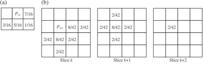
wherefare the error diffusion fractions from each corresponding location of the 2D filter, specifically 7/16, 1/16, 5/16, 3/16, respec-tively (seeFig. 2a).

Following this update, the procedure is repeated for each subse-quent location in turn. The proportions of the error diffused to adjacent pixels are determined heuristically and a typical filter for this in 2D is shown inFig. 2a[25]. An empty location in the fil-ter represents zero error diffused to this pixel.

3D error diffusion, while less common than 2D (as there are fewer potential applications), is a simple extension of the 2D pro-cess, where the error is diffused in 3D space to voxels around the current voxel. Again, the proportions of the original error to diffuse are determined heuristically and the filter used in this work is shown inFig. 2b[23]. In this case, Eq.(3)will consist of 20 loca-tions of Pxyzcorresponding to the locations and fractions shown inFig. 2b. In the 1D case, the error is diffused completely to the fol-lowing pixel.

Fig. 3presents a coarse numerical example that shows the ac-tual value changes resulting from following this procedure for a 2D case. A better visual binary representation would be possible with a higher resolution array. The application of 1D and 2D dith-ering methods to enable design of a cellular structure with variably sized cells is demonstrated with a larger example problem in the following section.

2.2. Cellular structure generation methodology

The method can be split into 3 main stages:

(1) Definition of functional grading.

(2) Error diffusion to generate dithered points of boundary and area.

(3) Application of connection scheme to generate structure cells.

2.2.1. Definition of functional grading

To generate a variable cellular structure, a continuous represen-tation of the desired functional variation is first required. This could be a result of a finite element analysis (FEA), for example, providing a temperature (for thermal problems) or stress (for structural problems) distribution, or a result of a density based Internal

cellular structure

Solid wall

Fig. 1.Cross section through an additively manufactured metal part containing a regular cellular structure.

(a) (b)

Slice k Slice k+1 Slice k+2

2/42 2/42

2/42

8/42 2/42

2/42

Pxyz 8/42 2/42

8/42 2/42

2/42 2/42 3/16

Pxy 7/16

5/16 1/16

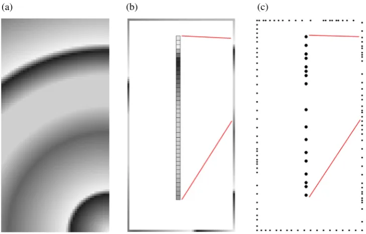
topology optimization[26]without penalisation of the intermedi-ate densities. However the functional variation is defined, it repre-sents the magnitude distribution of the analysis response. To demonstrate this method, the functional variation representation used is shown inFig. 4a.

2.2.2. Error diffusion to generate dithered points of boundary and area

This stage consists of two steps: the part boundaries are tack-led first, followed by the part area (or volume for a 3D part). In the 2D example, the boundary is identified as a single layer of pixels, as shown inFig. 4a. This layer is transformed into a single row of pixels per boundary using a boundary tracing method to preserve pixel order. For the part shown in Fig. 4, this gives a single one-dimensional row of variable greyscale pixels; this row is then dithered using 1D error diffusion. The dithered pixel row can then be transformed back to the correct shape, as shown inFig. 4c.

This boundary dithering stage serves two purposes. Firstly, it provides a more precise positional boundary than just using 2D dithering alone, as this does not necessarily place node points on the boundary. Secondly, it enables identification of the edges be-tween the node points that are to be constrained for stage 3 of the method where the connection schemes are applied.

Once the boundary points have been generated, the area can be tackled. Firstly, the area is reduced inwards by a pixel, as the boundary pixels have already been used. Secondly, by passing the filter fromFig. 2over this representation and diffusing the er-ror of binarisation accordingly, a point distribution is generated representing the cell spacing. The 1D (boundary) and 2D (area) dithered results are then combined to form a complete set (Fig. 5a). Due to the different filters used for the boundary and area, there is calibration required to ensure the resulting dithered points from the stages spatially correspond. This requires insight into how each filter affects the spacing of the dithering points which is

Pixel 1 Pixel 2 Pixel 3 Pixel 4 Pixel 5 Pixel 25

Error = 100 Error = -111 Error = 51 Error = 122 Error = -101 Error = -77

Fig. 3.Coarse numerical example showing the 2D filter being applied to a greyscale image. Each pixel is treated in turn and the error between the pixel and the corresponding binary image is diffused to adjacent pixels using the proportions defined by the filter.

(a)

(b)

(c)

investigated in Section 3. With this information the appropriate calibration parameter can be set.

2.2.3. Application of connection scheme to generate cellular structure cells

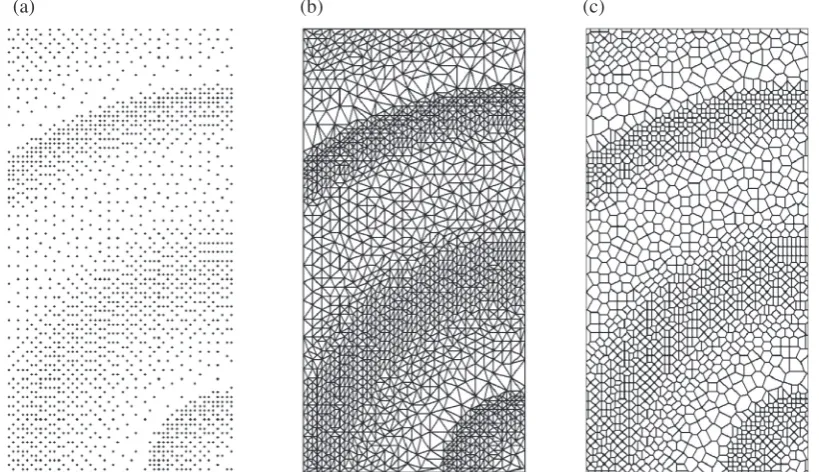
The third stage of the method is to apply a connection scheme to the dithered points to form the basis for the cellular structure. In this work, two example connection schemes were used: Dela-unay triangulation[27]and Voronoi tessellation[28,29]. The trian-gulation generates structural members that connect up the points whilst the Voronoi tessellation generates members that lie in the line/plane equidistant from the two nearest points. It is the edges of the polygons generated that form the member longitudinal axes onto which a geometric shape can be mapped, for instance a cylin-der. These cellular structures are shown inFig. 5and the mapping of cylindrical members to these edges, along with spherical end caps, is shown inFig. 6.

While the triangular cellular structure is more suited to applications where high stiffness is required as these cells are stretch-dominated [30], a Voronoi cellular structure, which has cells of a similar shape to those found in natural foams that should deform readily under load[2], is more suited to impact absorption applications as the cells are bending-dominated

[30].

3. Experiments to determine parameter relationships

The minimum and maximum cell sizes shown in the previous example are determined by two parameters: the image pixel/voxel resolution and greyscale value. Specifying real design limits for the cellular structure ensures that it can be optimised for a given load case, but this requires determination of the effect of these param-eters on the cell size range, which in turn enables local control over the generated node spacing and the overall quantity of generated nodes.

As mentioned in the previous section, a calibration is required between the boundary and area/volume dithers owing to the dif-ferent filters used. Without this calibration, there is a mismatch be-tween the minimum and maximum sizes of the resulting 1D boundary and 2D area geometries. This is also the case when com-bining 2D and 3D dithering stages in a 3D example. It is therefore useful to be able to link 1D, 2D and 3D dithering methods so that the required sizes of the cells throughout the area or volume and the boundaries are matched. With this in mind, experiments were carried out to investigate the effects of image pixel/voxel resolu-tion and greyscale value on the cell size range for both Delaunay and Voronoi connection schemes.

3.1. Test sample definition and analysis

A range of test 1D, 2D and 3D greyscale arrays were generated of varying image pixel/voxel resolution,Lbetween 10 and 100 pix-els in increments of 10, and greyscale level,Vbetween 0 and 240 in increments of 10. The greyscale ranges from 0 to 255, but an upper limit of 240 was used because in a pure white region, no dithered points would be generated. This means that the samples with grey-scale values above 240 there would be very few points or none at all to connect. On application to a real part, the boundary points would be included and allow connection but the samples did not include boundary points to reduce edge effects skewing the results. Each of the constant greyscale level samples was subjected to the relevant 1D, 2D or 3D error diffusion filter.

(a)

(b)

(c)

Fig. 5.(a) Error diffusion to generate dithered points of boundary and area, (b) Delaunay triangulation connection scheme and (c) Voronoi tessellation connection scheme to generate cellular structure cells.

Voronoi cell edge

Cylindrical member

Spherical end cap

Following dithering, in the case of the 1D samples, the average distance between the points was determined. In the case of the 2D and 3D samples, two connection schemes: Delaunay and Voronoi were used to generate either triangular/tetrahedral cells, or Voro-noi cells respectively. From these cells, the average element edge length, and area or volume was calculated. These measures are re-quired to control the sizes of the cells within the cellular structure. The results are presented in Sections3.2and3.3. The Voronoi cells on the boundary, i.e. those that have a vertex at infinity were ex-cluded from the calculations. In addition, vertices that were closer together than a specified distance were merged to avoid skewing the edge length results. For the Delaunay connection scheme, highly distorted (sliver) triangular/tetrahedral cells, generally located on the perimeter, were filtered out based on a radius tolerance. This filtering of edge effects increased the accuracy of the sample results.

3.2. Effect of sample parameters on cell edge length

To investigate relationships between the parameters and the cell edge length for the five cases: 1D, 2D and 3D for both Delaunay and Voronoi connection schemes, a surface defined by Eq.(4)was fitted to the sample results using a nonlinear least squares method as implemented in MATLAB using variable bounds determined from parametric studies. The relationships between the two parameters,VandL, and the mean cell area (2D) or cell volume (3D) were found to be a close fit to Eq. (4)as demonstrated by the goodness of fit measures inTable 1. The corresponding coeffi-cients for the five cases are also presented inTable 1. It was found that there was a power relationship betweenLand edge length and there was a double exponential relationship betweenVand edge length.

It can be seen fromFig. 7that in the Voronoi cell case, the data is not as smooth as the Delaunay method and there are several peaks over the range of parameterV. The error between the fitted surface and data is shown by the goodness of fit measures in

Table 1. This artefact is investigated further in Section3.4.

A¼10^

ððc5Lc6þc7Þ ðc1ec2VÞ þ ðc3ec4VÞÞ ð4Þ

3.3. Effect of sample parameters on cell size

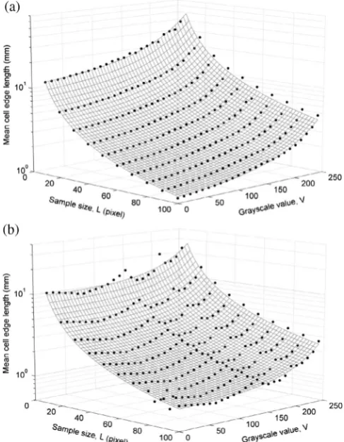
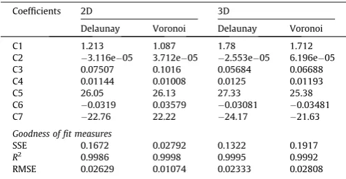
The same samples were used to evaluate the effect on the cell size, specifically the area in 2D and volume in 3D. Results for the 2D cases for Delaunay and Voronoi connection schemes are shown in Fig. 8. Similar to the edge length results, the relationships betweenVand Land the mean cell area or volume were found to be a close fit to Eq.(4)as demonstrated by the goodness of fit

measures inTable 2. In contrast to the edge length results, the Voronoi results are more closely represented by the fitted surface.

3.4. Variability of results

The variability in edge length and area was investigated for both the Delaunay and Voronoi connection schemes. Each greyscale integer point was evaluated for a fixed sample size, the results of which are shown inFigs. 9and10. The mean is represented by the solid central line and the standard deviation is shown by the grey region either side. The inset squares show the sample cells for different regions over the greyscale range.

Across both sets of samples, the variability in the member edge length was more significant than that of the cell area. For the area, the variability dropped to zero or close to zero at several positions along the greyscale range. At these regions, the cellular structure consists of identical or very similar size cells as can be seen from the samples shown. For the Delaunay results, as the triangular cells are not equilateral this decrease in variability is only marginally apparent in the edge length variability results. However, for the Voronoi results, the reductions in variability correspond to square cells which do have equal edge lengths.

Also of interest in the Voronoi edge length results is the increase in the mean when the variability decreases. Very short cell edges were filtered out before analysis by merging vertices, but due to the greater variation in cell shape (as can be seen inFig. 11) com-pared with Delaunay, there is still more variation in edge length for Voronoi cells. This means that it will be more difficult to correlate the member length at the boundary and area or volume of cells generated using the Voronoi connection scheme compared with Delaunay.

Table 1

Fitted surface coefficients and goodness of fit measures for all cases considered.

Coefficients 1D 2D 3D

Delaunay Voronoi Delaunay Voronoi

C1 99.23 0.6795 0.8076 1.447 0.4874

C2 0.000518 0.0001574 0.0001044 4.216e05 0.0004864 C3 0.1475 0.03448 0.01034 0.02166 0.0286 C4 0.007842 0.01186 0.01577 0.01226 0.01098

C5 22.71 24.95 24.28 23.9 25.16

C6 0.0001954 0.02899 0.02562 0.01346 0.05

C7 22.69 21.77 21.64 22.48 20.43

Goodness of fit measures

SSE 0.2882 0.06547 0.3715 0.02223 0.1379

R2 _{0.9917 0.9979 0.9867 0.9992 0.9956}

RMSE 0.03444 0.01645 0.03918 0.009566 0.02382

3.5. Applicability of investigated relationships to cellular structure design

3.5.1. Cell area/volume control

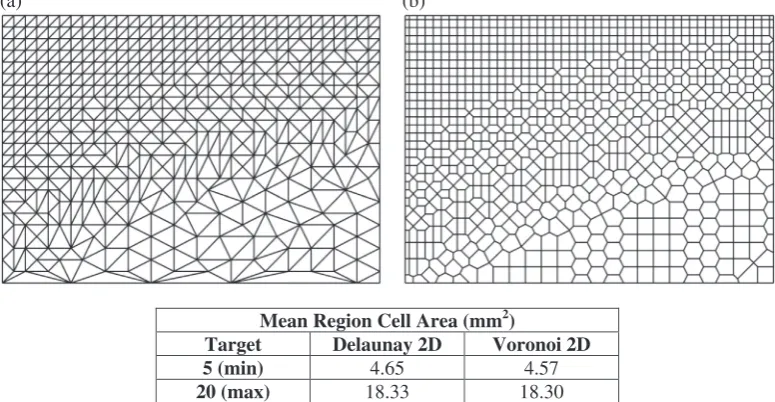
To evaluate the use of the defined relationships between the cell area or volume and the two parameters discussed above, a demonstration example was used (Fig. 12) for both Delaunay and Voronoi connection schemes.

L¼ log10Ac3e

c4V

c1ec2Vc₅

c7 c5

1=c6

ð5Þ

To satisfy the requirement of a minimum cell area,A, of 5 mm2_in

the black region (V= 0), Eq.(4) was rearranged to obtain Eq.(5), which can then be used to calculate the input image pixel/voxel resolution,L required to achieve our desiredA. For the Delaunay example,Lwas calculated to be 34. This image size can then be used

to satisfy the second requirement of a maximum cell area, A of 20 mm2_{. It is not possible to rearrange Eq.(4)to isolate the}

gray-scale parameter, V, so an iterative procedure can be used to find the closest value ofAto the target by varyingVusing the previously calculatedLfrom the determination of the minimum cell size. In this case, the difference was minimised using the simplex search Fig. 8.Effect of parameters on mean cell area for (a) 2D Delaunay connection

scheme, and (b) 2D Voronoi connection scheme.

Table 2

Fitted surface coefficients and goodness of fit measures for all cases considered.

Coefficients 2D 3D

Delaunay Voronoi Delaunay Voronoi

C1 1.213 1.087 1.78 1.712

C2 3.116e05 3.712e05 2.553e05 6.196e05

C3 0.07507 0.1016 0.05684 0.06688

C4 0.01144 0.01008 0.0125 0.01193

C5 26.05 26.13 27.33 25.38

C6 0.0319 0.03579 0.03081 0.03481

C7 22.76 22.22 24.17 21.63

Goodness of fit measures

SSE 0.1672 0.02792 0.1322 0.1917

R2

0.9986 0.9998 0.9995 0.9992

RMSE 0.02629 0.01074 0.02333 0.02808

Mean

-1SD +1SD

Mean

-1SD +1SD

(a)

(b)

Fig. 9.2D Delaunay variability for (a) edge length, and (b) cell area.

Mean

-1SD +1SD

Mean -1SD +1SD

(a)

(b)

method[31]as implemented in MATLAB, and the value forVwas found to be 193.

This updated grayscale value is accommodated by modifying the input image grayscale distribution by multiplying by the differ-ence (grayscale darkening/lightening) between the twoV values (for 5 mm2_{and 20 mm}2_{). Because the lowest value of the range}

is 0, the previously defined minimum cell size is unchanged. The desired extreme element sizes are therefore defined by modifying the image size for the minimum size and then modifying the grey-scale level for the maximum size. Both the Delaunay and Voronoi connection schemes were evaluated for these two size require-ments and the results are shown inFig. 13. It was found that in both cases, there was an underestimation of the cell area in both the minimum and maximum regions. For the Delaunay case these errors were 7% and 8.4%, and for Voronoi, 8.6% and 8.5%. This error is due to deviation of the fitted surface from the data; however, because it is reasonably consistent, it could be empirically com-pensated for.

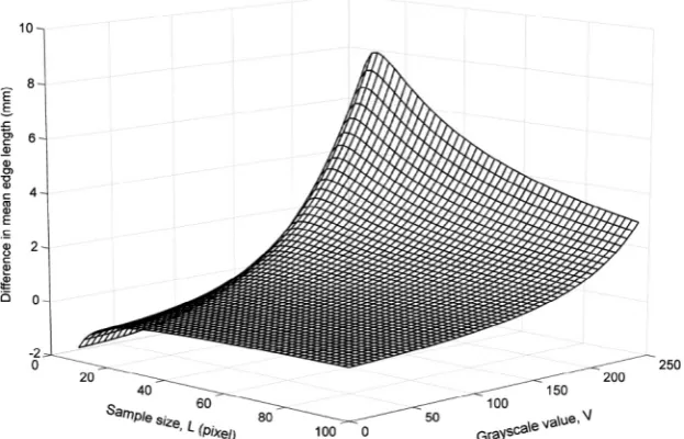
3.5.2. Matching boundary to area/volume edge lengths

As the boundary and area or volume dithering stages are carried out independently using different error diffusion filters, the result-ing spacresult-ing of the dithered points are unlikely to match. This mis-match can be seen inFig. 14which shows the fitted surfaces for the 1D case and 2D Delaunay case, with the only matching instance shown by the plotted intersection curve. The difference as shown inFig. 15can be compensated for by modifyingVwhilst keeping

Las previously calculated.

4. Discussion

4.1. Cellular structure member orientation

Depending on the application of the cellular structure, local control of member orientation can be beneficial, primarily for load bearing applications. However, the error diffusion filter does not inherently allow local orientation control for two reasons: firstly, the filter is passed row by row across the part and does not follow its geometric profile, and secondly, the Delaunay triangulation and Voronoi tessellation connection methods do not handle direction constraints. The end result of this is likely to be a sub-optimal solu-tion and so the approach may be more suited to applicasolu-tions where the orientation of members has less of an effect or is not known in advance, potentially for heat dissipation and impact absorption applications.

There are some instances of the use of a variable diffusion filter to allow local control of the dithered result, for example, to empha-sise edges[32,33]. A similar approach could potentially be adopted to improve upon the current method by taking account of principal stress tensors or force flow directions to influence the structural member orientation by making a corresponding adjustment to the error diffusion filter. However, it is difficult to see how this would have a significant effect on the member orientation, Fig. 11.Sample Voronoi cells demonstrating the significant variability of cell shape.

Target:

5 mm

Target:

20 mm

Fig. 12.Specification of targets for sizing control evaluation.

(a)

(b)

Mean Region Cell Area (mm

)

Target

Delaunay 2D

Voronoi 2D

5 (min)

4.65

4.57

20 (max)

18.33

18.30

especially with the Voronoi connection scheme where members are generated around the dithered points.

An alternative approach could be to identify members that exist in a particular orientation and increasing the cross sectional dimensions of these members, while also reducing the dimensions of members in differing orientations.

4.2. Boundary dithering

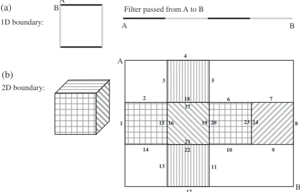
In the example shown in Section2.2, the boundary dithering is carried out using a 1D filter. This requires that the boundary pixels be transformed into a straight path as shown inFig. 16a. The filter is then passed along this path from the start to the end diffusing the pixel error accordingly. However, because the start and end of the path are no longer adjacent, these adjacent pixels are not in-cluded in the error diffusion processing causing incorrect dithering to some extent. In the specific case presented in Section2.2, this is not of significance as the greyscale values of the pixels at A and B are consistent, but in other cases this may not be the case.

This issue is more complex when tackling 3D problems as the boundaries are surfaces and so require 2D error diffusion. For a simple shape such as the cube shown in Fig. 16b the process of transforming the boundaries to 2D is straightforward, but for a more complex shape, mapping procedures[34]could be applied. In the same way that for the 1D case, the adjacent pixels A and B are no longer adjacent following transformation, in the 2D case several adjacent edges are no longer adjacent following transfor-mation. For instance, inFig. 16, edges 2 and 3 are separated while edges 15 and 16 remain adjacent. The error diffusion filter is passed over the rectangular region surrounding the unwrapped boundary surface from A to B in a row by row fashion and so does not account for the separated adjacent edges in the process.

5. Summary and conclusions

This paper has presented a novel method of generating a func-tionally graded cellular structure based on a functional variation representation input. The spatial variation in the area/volume of

1D filter 2D filter with

Delaunay connection scheme

Intersection curve

Fig. 14.1D case and 2D Delaunay case edge length fitted surfaces, with intersection curve shown.

the cells is achieved using error diffusion to convert a continuous tone image into binary form. It is not claimed that this is an overall optimal solution, but it is an efficient and novel way to create a functionally graded cellular structure with a small number of de-sign variables.

The effect of the two parameters, image pixel/voxel resolution and greyscale value on the resulting cell edge length and area/vol-ume was investigated. For both the edge length and area/volarea/vol-ume results, Eq.(4)represented the mean data well. In the case of the Voronoi edge length results, the variation in the cell shape causes peaks at certain parameter combinations resulting in a worse fit. At these combinations, the edge lengths of the cells are equal and so the variability becomes zero and the mean value increases relative to the other combinations.

The fitted relationships were applied to an example, where the target was to control the minimum and maximum cell size for the two connection schemes. In both cases there was approximately an 8% underestimation of cell area for both minimum and maximum target regions. A comparison of the edge length results for the boundary and area was also made, and a step outlined for adjusting the boundary results to ensure a closer match between the edge lengths.

The limitations of using this error diffusion based approach were discussed, the main ones being the difficulties of specifying structural member orientation and the complexities of error diffu-sion of boundaries especially when tackling 3D problems. The first of these issues could be addressed by using a variable diffusion fil-ter or by applying local dimensional changes based on structural member orientation. The second of these issues could be addressed to some extent by using mapping techniques, but a more advanced filtering process where edges that are adjacent are considered simultaneously would be useful.

To extend the proposed method to 3D, a volumetric functional variation representation is required as an input, which can be ob-tained by taking slices through a 3D FEA mesh fringe at the same resolution as the in plane dimensions. It is important that these resolutions are the same or the cellular structure will be distorted in a particular dimension. As would be expected, a 3D error diffu-sion filter such as that shown inFig. 2b should be used. A con-strained 3D Delaunay algorithm capable of handling non-convex point envelopes and connecting interior and boundary dithered points could be used to generate the 3D cellular structure.

Acknowledgments

The authors would like to thank the UK Technology Strategy Board (TSB) and the UK Engineering and Physical Sciences Research Council (EPSRC) for funding this work.

References

[1]Wadley HNG. Multifunctional periodic cellular metals. Philos Trans. Ser A Math Phys Eng Sci 2006;364(1838):31–68.

[2] Brennan-Craddock J. The investigation of a method to generate conformal lattice structures for additive manufacturing. Loughborough University; 2011. [3]Brennan-Craddock J, Brackett D, Wildman R, Hague R. The design of impact absorbing structures for additive manufacture, modern practice in stress and vibration analysis 2012 (MPSVA 2012). J Phys: Conf Ser 2012;382:012042. [4]Gu S, Lu TJ, Evans AG. On the design of two-dimensional cellular metals for

combined heat dissipation and structural load capacity. Int J Heat Mass Transfer 2001;44(11):2163–75.

[5]Ozmat B, Leyda B, Benson B. Thermal applications of open-cell metal foams. Mater Manuf Processes 2004;19(5):839–62.

[6]Seepersad CC, Dempsey B, Allen JK, Mistree F, McDowell DL. Design of multifunctional honeycomb materials. AIAA J 2004;42(5):1025–33. [7]Wadley H, Queheillalt T. Thermal applications of cellular lattice structures.

Mater Sci Forum 2007;539–543:242–7.

[8] Kumar V, Manogharan G, Cormier D. Design of periodic cellular structures for heat exchanger applications. In: Proceedings of the solid freeform fabrication symposium. Texas; 2009. p. 738–48.

[9] Cook D, Newbauer S, Pettis D, Knier B, Kumpaty S. Effective thermal conductivities of unit-lattice structures for multi-functional components. In: Solid freeform fabrication symposium. Texas; 2011. p. 696–18.

[10] Cook D, Newbauer S, Leslie A, Gervasi V, Kumpaty S. Unit-cell-based custom thermal management through additive manufacturing. In: Proceedings of the solid freeform fabrication symposium. Texas; 2012. p. 121–37.

[11]Evans AG, Hutchinson JW, Fleck NA, Ashby MF, Wadley HNG. The topological design of multifunctional cellular metals. Prog Mater Sci 2001;46(3– 4):309–27.

[12]Baumers M, Tuck C, Hague R. Realised levels of geometric complexity in additive manufacturing. Int J Prod Dev 2011;13(3):222–44.

[13] Brackett D, Ashcroft I, Hague R. Topology optimization for additive manufacturing. In: 22nd annual international solid freeform fabrication symposium. Austin, Texas; 2011. p. 348–62.

[14] Aremu A, Brackett D, Ashcroft I, Wildman R, Hague R, Tuck C. An adaptive meshing based BESO topology optimisation. In: 9th World congress on structural and multidisciplinary optimization (WCSMO-9). Shizuoka, Japan; 2011.

[15]Aremu A, Ashcroft I, Wildman R, Hague R, Tuck C, Brackett D. The effects of Bi-directional evolutionary structural optimization parameters on an industrial designed component for additive manufacture. Proc Inst Mech Eng Part B J Eng Manuf 2012;227:794–807.

[16] Watts DM. A genetic algorithm based topology optimisation approach for exploiting rapid manufacturing’s design freedom. Loughborough University; 2008.

Filter passed from A to B

A B 1D boundary: 2D boundary: A B A B 1 2 5 6 8 7 3 9 10 11 4 12 13 14

15 16 19 20

18 17 21 22 23 24

(a)

(b)

[17] Wang H, Rosen DW. Parametric modeling method for truss structures. In: Proceedings of DETC’02 2002 ASME design engineering technical conferences and computers and information in, engineering conference; 2002. p. 1–9. [18] Gervasi VR, Stahl DC. Design and fabrication of components with optimized

lattice microstructures. In: Proceedings of solid freeform fabrication symposium. Texas; 2004. p. 838–44.

[19] Alliez P, Desbrun M, Meyer M. Efficient surface remeshing by error diffusion; 2002.

[20]Brankov JG, Wernick MN. Content-adaptive mesh modeling for fully-3D tomographic image reconstruction. In: Proceedings of international conference on image processing. IEEE; 2002. p. 621–4.

[21] Brankov JG, Yang Y, Wernick MN. Accurate mesh representation of vector-valued (colour) images. In: Proceedings of international conference on image processing (ICIP); 2003. p. 3–6.

[22]Sarkis M, Diepold K. Content adaptive mesh representation of images using binary space partitions. IEEE Trans Image Process: Publ IEEE Signal Process Soc 2009;18(5):1069–79.

[23] Lou Q, Stucki P. Fundamentals of 3D halftoning. In: 7th International conference on electronic publishing, EP’98 Held jointly with the 4th international conference on raster imaging and digital typography, RIDT’98. St. Malo, France; 1998. p. 224–39.

[24] Chau WK, Wong SKM, Wan SJ. A critical analysis of dithering algorithms for image processing. In: IEEE Region 10 conference on computer and communication systems. Hong Kong; 1990. p. 309–13.

[25]Floyd R, Steinberg L. An adaptive algorithm for spatial grey scale. Proc Soc Inf Disp 1976;17(2):75–7.

[26]Bendsoe MP. Optimal shape design as a material distribution problem. Struct Optim 1989;1:193–202.

[27]Delaunay B. Sur la sphère vide. Izvestia Akademii Nauk SSSR, Otdelenie Matematicheskikh i Estestvennykh Nauk 1934;7:793–800.

[28]Dirichlet GL. Über die Reduktion der positiven quadratischen Formen mit drei unbestimmten ganzen Zahlen. Journal für die Reine und Angewandte Mathematik. 1850;40:209–27.

[29]Voronoi G. Nouvelles applications des parametres continus ä la theorie des formes quadratiques. Journal für die reine und angewandte Mathematik. 1908;134:198–287.

[30] Ashby MF. The properties of foams and lattices. Philos Trans R Soc A London 2006;364(1838):15–30.

[31]Lagarias JC, Reeds JA, Wright MH, Wright PE. Convergence properties of the Nelder–Mead simplex method in low dimensions. SIAM J Optim 1998; 9(1):112–47.

[32]Chang J, Alain B, Ostromoukhov V. Structure-aware error diffusion. ACM Trans Graphics (TOG) 2009;28(5).

[33]Garg P, Gupta A, Srivastava MC, Gupta A, Agarwal N. Edge-directed error diffused digital half-toning: a steerable filter approach. Int J Signal Process Image Process Pattern Recogn 2009;2(3):43–56.