Magnetic support of stellar slingshot prominences

Magnetic support of stellar slingshot prominences

Rose F. P. Waugh

and Moira M. Jardine

SUPA, School of Physics and Astronomy, University of St Andrews, North Haugh, St Andrews KY16 9SS, UK

Accepted 2018 November 16. Received 2018 November 15; in original form 2018 September 20

A B S T R A C T

We present models for the magnetic support of the ‘slingshot prominences’ observed in the coronae of rapidly rotating stars. We calculate mechanical equilibria of loops in a spherical geometry. Prominence-forming loops are found first for dipolar and quadrupolar stellar fields that are fully closed. Equilibria are then found within the stellar wind for a dipolar field that becomes open beyond a given radius. We identify two physical processes that may produce gaps in the distribution of prominence heights: the location of this opening radius, and the behaviour of the buoyancy force. The buoyancy may differ from one prominence-bearing loop to another if they are at different temperatures, thus potentially smearing out any gap in observed height distributions. We produce synthetic prominence distributions and compare to the observations of two well-observed stars: AB Doradus and Speedy Mic. The model recovers the more compact prominence distribution observed for Speedy Mic and reproduces better the overall shape of the height distributions for both stars when the opening radius is beyond the co-rotation radius.

Key words: stars: individual: AB Dor – stars: low mass – stars: magnetic field.

1 I N T R O D U C T I O N

Prominences are cool condensations of neutral hydrogen, embed-ded within a hot corona. These features are perhaps best known as dark filamentary structures against the solar disc, or bright material protruding above the solar limb. They are not restricted to our Sun, however, having been observed on many other stars albeit not in the same resolution. Since they are confined by the magnetic field, they trace out the coronal magnetic field structure. This makes them use-ful since the current method of generating such information involves extrapolation of the stellar surface magnetic field, gained from Zee-man Doppler imaging. These features could have consequences for stellar evolution. Ejection of active prominences is thought to be a

method of stellar angular momentum and mass-loss (Hussain2013).

While the effect of these features will likely be small while com-pared to the stellar wind, it could be non-negligible (Aarnio, Matt &

Strassun2012; Cranmer2017; Odert et al.2017). Ejections could

also be responsible for loss of helicity from the system, as on the

Sun (Low2006,1994; Wang, Zhou & Zhang2004). Development

of any nearby planets, and their ability to harbour life, could also be influenced by ejection of these condensations. Impact of ejected prominences with an exoplanet could lead to geomagnetic storms, compression of the planetary magnetosphere by shock waves

(Gon-zalez et al.1994), and atmospheric erosion due to the stripping of

the planetary atmosphere by frequent impacts (Khodachenko et al.

2007).

_{E-mail:rw47@st-andrews.ac.uk}

The first suggestion of prominences on other stars came from bi-nary systems where, as one star eclipsed its partner, the light from the background star was used to probe the atmosphere of the foreground

star (Schroder1983). When analysing the spectra, unexplained

ab-sorption features were found immediately preceding or subsequent to the rotation phase at which the eclipse took place. These transient absorption features had been seen to reoccur on consecutive peri-ods, sometimes dimming or brightening in intensity. This suggested the material being supported in co-rotation could, in some cases, be reasonably stable. The star SS Bootis was observed by Hall et al.

(1990) in 1987 and 1988, and then again in 1992 by Hall & Ramsey

(1992) as part of a larger scale study into these features. The authors

reported the existence of a feature at the same height in both works. They suggested that either the feature was incredibly stable or that this could be a particularly stable point within the magnetic field, with condensations being repeatedly trapped at this point.

Similar absorption features were subsequently seen on the rapidly

rotating, K0V type star, AB Doradus (Cameron & Robinson1989).

They were observed as transient dips in the Hα profiles,

cross-ing the disc in a matter of hours and sometimes reappearcross-ing on consecutive nights. This behaviour was consistent with absorbing material located around two to nine stellar radii from the stellar rotation axis and co-rotating with the star (Cameron & Robinson

1989). Thought to be held in co-rotation by the coronal magnetic

field, these features were coined ‘slingshot prominences’ (Cameron

1996; Steeghs et al.1996). While AB Dor may be the best observed

rapid-rotator prominence host, prominences have been observed

on multiple rapidly rotating stars(Dunstone et al.2006a,b; Jeffries

1993; Byrne, Eibe & Rolleston1996; Barnes et al.1998; Cameron &

2018 The Author(s)

Woods1992; Barnes et al.2000; Leitzinger et al.2016; Skelly et al.

2008,2009,2010; Eibe1998).

Slingshot prominences have also been seen on M dwarfs, for

example V374 Peg (Vida et al.2016), a fully convective, ultrafast

rotator. Later, Stauffer et al. (2017) found 19 M dwarfs exhibiting

prominence-like absorption dips within K2 light curves. Variations in flux that repeated at the same phase on each rotation were consis-tent with cloud condensations trapped in co-rotation. These stellar prominences on rapidly rotating stars are rather different to their solar namesakes. They typically occult a larger area of the stellar surface than solar prominences, are 10–100 times larger in mass and can be found significantly further out from the stellar rotation

axis (Cameron1999).

Previously, Jardine & Cameron (1991) published a model to

de-scribe prominence formation within the equatorial plane of such rapidly rotating stars. The authors showed that for an isothermal atmosphere in hydrostatic equilibrium, a cool loop may reach a mechanical equilibrium whereby a prominence may be supported. This is achieved through the balance of the gravitational, Lorentz

and centrifugal forces. Ferreira (2000) later published a paper

dis-cussing the stability of such prominences and Jardine & van

Bal-legooijen (2005) found available equilibria within the stellar wind.

This removed the requirement for the stellar corona to be closed up to the large heights from the stellar surface at which promi-nences are typically observed. More recently, Villarreal D’Angelo,

Jardine & See (2018) categorized which low-mass stars could be

capable of supporting such prominences. By comparing whether the Alfv´en radii of stars were inside or outside of the co-rotation radius, the authors were able to determine if prominence formation could be supported. This work adopted terms such as ‘centrifugally supported magnetospheres’ and ‘dynamical magnetospheres’,

pre-viously applied in the context of massive stars (Petit et al.2013;

Owocki et al.2016). These terms are used to distinguish between

distinct types of phenomena by which material is either supported against gravity or will fall back to the stellar surface. This idea of supporting material beyond the Keplerian co-rotation radius under

force balance has been extensively discussed (Cassinelli et al.2002;

Townsend & Owocki2005; ud-Doula, Owocki & Townsend2008).

In this paper we aim to extend the model developed by Jardine &

van Ballegooijen (2005) of prominence formation in a locally

two-dimensional, Cartesian geometry. Here we extend their model to a spherical coordinate system, describing the low-order multipoles that dominate the magnetic field structure at the heights of several stellar radii at which these prominences are supported. Most im-plementations of the Zeeman–Doppler imaging technique express the recovered fields in terms of spherical harmonics and so can pro-vide insight into the contribution of the different modes (Donati &

Landstreet2009). In particular, we aim to show that solutions for

mechanical equilibria in this geometry replicates the results of

Jar-dine & van Ballegooijen (2005) for prominence formation within

the open field region. We consider the influence of the background field topology, as well as the impact of allowing the field to become open above and below the co-rotation radius. Since there is no direct observational evidence of the location at which the stellar magnetic field becomes open, we consider both cases here.

2 M E T H O D

The physical scenario that we model is that of cooled loops embed-ded in a hot external magnetic field. We choose both dipolar and quadrupolar external fields, and in both cases the magnetic axes lie in the equatorial plane of the star. In the case of the dipolar field,

Figure 1. Diagrams of the external magnetic fields used: (top) dipolar, (middle) quadrupolar, and (bottom) dipolar with the addition of a source surface (red dashed line). The stellar surface is shown by the orange circle; this is used throughout the figures in the rest of this paper. The magnetic axis is aligned along the horizontal axis.

we also investigate the impact of allowing the field to be open

be-yond some radius, known as the ‘source surface’rs(Altschuler &

Newkirk1969). We focus only on the equatorial plane as shown

in Fig.1where the field structures are defined by the following

equations:

Be=B0

2 cosφ

r3

ˆ

r+

sinφ

r3

ˆ

φ

, (1)

Be=B0

3(3 cos(φ)2₋₁₎

2r4

ˆ

r+

3 cos(φ) sin(φ)

r4

ˆ

φ

, (2)

and

Be=B0

2 cosφ r3

r3_+2r3 s

R3 +2rs3

ˆ r+ sinφ r3

−2r3_+2r3 s

R3 +2r3s

ˆ

φ

(3)

for dipolar and quadrupolar fields and a dipolar field that is open

beyondrs(Jardine, Cameron & Donati2002a).B0is the maximum

magnetic field strength at the stellar surface andφrepresents the

angle, measured from the dipole axis (φ = 0), measured in the

equatorial plane.

Within this model, we assume that the loops in question are isothermal and ‘thin’, so that any internal quantities do not vary across the width of the flux tube. In assuming the thin flux tube approximation we also assume that the area of the flux tube is much smaller than the pressure scale height squared, and that the tube does

not significantly disturb the background field (Parker1975; Spruit

1981). They must be in pressure balance with their environment

B2 i =B

2

e +2μ(pe−pi), (4)

whereμrepresents the permeability of free space and pthe gas

pressure. The subscripts e and i refer to external and internal quan-tities, respectively. Then, in order to determine the shape of the loops, force balance must be solved along and across the magnetic field lines.

We assume our system to be in hydrostatic equilibrium with no flows, therefore the forces acting on the loop can be modelled by

0= −∇p+(j×B)+ρg, (5)

where∇pis the gradient of the gas pressure, (j×B) is the Lorentz

force, ρ represents the gas density (defined by the equation of

state,p=KBTρ/m, where symbols have the usual meanings and

mrepresents the mean molecular mass) andgis the gravitational

acceleration. Decomposing the Lorentz force into magnetic pressure and tension terms yields

0= −∇p+(B.∇)B

μ− ∇

B2

2μ

+ρg. (6)

We construct our equations in the co-rotating frame, combining the centrifugal and gravitational forces into an ‘effective gravity’ term,

gef=

−GM

r2 +ω

2_r

ˆ

r (7)

which replacesgin equation (6) and whereωis the stellar rotation

rate. The nature of this equilibrium can be most clearly seen by combining equations (4), (6), and (7) to give

0= −(ρe−ρi)gef− ∇

B2 e

2μ

+(Bi.∇) Bi

μ, (8)

where the tension of the loop balances the combined effects of buoyancy and the gradient of the external field. The loop tension is of course determined by its shape. In order to determine this, we

decompose equation (6) into components parallel (ˆs) and

perpen-dicular ( ˆn) to the path of the magnetic field line, we define the unit

vectors

ˆ

s= 1

r2+_(r)2(r

_{, r) (9)}

ˆ

n= 1

r2+_(r)2(−r, r

_{). (10)}

Parallel to the magnetic field line, there is no Lorentz force and equation (6) simplifies to

∂p

∂r =gefρ, (11)

where we have taken the gas pressure (p0at the stellar surface) to

be independent ofφ. This defines the gas pressure variation with

distance from the surface

p=p0exp

m KBT

r

R gef(r)dr

. (12)

The functionH(r) can be defined such that

H(r)≡ m

KBTe

−GM

r

1− r

R

+ ω2 2

r2−R2

, (13)

which yields a more compact form of equation (12)

pi(r)=p0iexp(H(r)), (14)

wherep0iis the base pressure inside the flux tube.

The component of equation (6) perpendicular to the magnetic field is

0= −∇p.nˆ+

B2∂sˆ ∂s

·nˆ+ ∇

B2

2μ

·nˆ+ρg.nˆ, (15)

where

∂

∂n=nˆ.∇ =

1

r2+_(r)2

−r ∂ ∂r +r

∂

∂φ

(16)

and

∂ˆs

∂s =(ˆs.∇)ˆs=

(rr−r2_−2(r)2₎

(r2+_(r)2₎₎3/2 nˆ. (17)

Therefore, the component of the force balance equation perpendic-ular to the magnetic field line simplifies to

2B2

ir(r

2_+2(r)2_−rr)

(r2_+(r)2₎ =

−r2∂ ∂r +r

∂

∂φ

Bi2. (18)

Combining equation (18) with pressure balance as expressed in

equation (4), the path of the cooled field line,r(φ), can be calculated

and the loop shape plotted.

3 L O O P S H A P E S

In exploring the factors that determine the loop shapes we use, as an example, the stellar parameters for a specific star. We choose

here to take the parameters of AB Doradus:R=0.96 R,M=

0.86 Mand period of 0.514 d (Innis et al.1988; Guirado et al.

2010,2011). We assume the background corona has a temperature

of 107_{K (Hussain et al.2005; Close et al.2007).}

3.1 Pressure variation with height

In order to achieve an equilibrium for these loops, two constraints must be satisfied: the internal gas pressure must not become too large relative to its environment and the forces perpendicular to the loop must be in balance. The first constraint is such that in

equation (4),B2

i >0.B 2

ewill always be positive, however (pe−pi)

may be negative ifpibecomes too large. If this difference is small,

this need not be a problem for equilibria, so long asB2

e is large

enough to balance it. The external field strength decays with height, however, and so beyond a certain value, this will no longer be true and no equilibria may be found. The second constraint corresponds to equation (18), where the magnetic tension (shown on the left-hand side) must be equal to the magnetic pressure gradient (shown on the right-hand side).

Considering the component of force balance along the field line yields equation (14). From this it can be seen how gas pressure

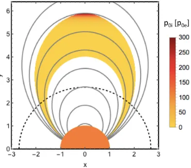
Figure 2. Example of the variation of pressure (pi) with height within these

cool loops. This is scaled to the external pressure (p0e) at the loop footpoints.

This example was calculated with parameters:Te=107K,β=10−7,p0i=

2p0e,Ti=0.03 Te. The background field into which this loop would be

embedded is shown in grey. The co-rotation radius is shown by the black, dashed line.

varies with height, noting that the sign ofH(r) depends on distance

from the stellar rotation axis, taking a negative value at low radii and a positive value at high radii. This is dependent on the stellar rotation rate and thus from here the effects of rapid rotation can be seen. Due to the rapid rotation, gas above the co-rotation radius

of the star is driven outwards into the tops of loops. Fig.2shows

an example of the increase in gas pressure with height beyond the co-rotation radius within a magnetic loop. This is similar to the

results from Jardine & Cameron (1991) in a Cartesian geometry,

with pressure dropping with height below the co-rotation radius and rising beyond it, as per equation (14).

3.2 Varying the field topology

We first choose to vary the field topology, applying both a dipolar and quadrupolar external magnetic field.

An external dipolar field is applied and using equation (18), combined with pressure balance (equation 4), solutions can be found for a set of mechanical equilibria. The magnetic field strength is scaled to the external value at the stellar surface. The top panel of

Fig.4shows the external field in grey on the right-hand side of

the figure and some example solutions shown by the blue loops on the left-hand side. The loop shapes deviate from the background field significantly at large heights where the gas pressure dominates over magnetic pressure. The effect of the centrifugal force acting to stretch out the cool, mass-loaded loops can be clearly seen. A

‘Height-Width plot’ shown in the bottom panel of Fig.4shows the

family of solutions, with ‘height’ and ‘width’ defined in Fig.3. In

this parameter regime, the footpoint separation of the cool loops increases with summit height, following the external field at low radii before deviating from the external field and becoming smaller with increasing loop height as the magnetic field strength drops to zero. It should be noted that ‘width’ here refers to the angular distance between the loop footpoint and loop summit.

Here we use a very small value ofβfor illustrative effects, to

exaggerate the distortion of the loops by the centrifugal effects. When calculating the prominence distributions generated from this model and comparing them to observations, we chose a more

real-Figure 3. Figure showing the definitions of ‘loop height’ (or ‘distance from the rotation axis’) and ‘loop width’.

istic value ofβ. This value ofβwas viewed as realistic since the

average field strength on AB Dor is observed to be around 10G and

the base pressure can be estimated usingp=κB2₌₁₀−5.5_B2

(Jar-dine et al. 2002b), with B in Gauss. Thus using β = 2μp/B2 _a

value of 10−3was seen as reasonable. The effects of varying the

base plasma beta value on the maximum loop height was discussed

by Jardine & Cameron (1991), where smallerβvalues were found

to allow taller loops. The cooled loops shown in all the examples throughout this paper are only cooled to a tenth of the external field,

orTi= 106K. This was chosen purely for ease of calculation as

dropping the internal temperature can make solutions increasingly difficult to solve for. The effects of varying temperature on these hydrostatic solutions has been discussed previously by Jardine &

van Ballegooijen (2005) and thus was not examined in detail here.

Jardine & van Ballegooijen (2005) considered the effects of

de-creasing the loop temperature on maximum loop height and found

the maximum loop height did not vary significantly betweenTi=

106_{K andT}

i=104K.

An external quadrupolar field is also applied and by the same method, solutions can again be found for a set of mechanical

equi-libria. An example is shown in Fig.5for the same parameters as the

above dipolar case. Once again, the cool internal loops are shown in blue on the left-hand side of the top panel and the external field shown on the right-hand side in grey. As with the dipolar field, the family of solutions for the cooled loops follows the external field at low heights, before deviating and becoming taller and thinner with increasing summit height. Naturally, these loops are constrained to a smaller angular extent by the geometry of the system, with the

loops now being constrained to π

4 radians rather than

π

2 radians.

This is seen clearly by comparison of the height versus width plots for the two cases.

The maximum attainable loop height can be calculated by con-sidering the point at which the magnetic field of these cool loops

(Bi) vanishes, i.e. where the footpoint separation of the loop is equal

to zero. These were found to ber=5.98 Randr=5.34 Rfor the

dipole and quadrupole, respectively. Beyond this height, the tension force cannot increase enough to balance the gradient in magnetic pressure and buoyancy forces, and thus no more hydrostatic solu-tions can be found.

3.3 Allowing the field to become open at large heights

Choosing a background field that has a source surfaceabovethe

co-rotation radius, and solving for the shapes of cool loops embedded

Figure 4. Background (grey) and cooled (blue) loops and the corresponding variation of loop height with footpoint separation (or width) for parameters:

Te=107K,Ti=Te/10,p0i=2p0eand a plasmaβat the loop footpoints of β=10−7_{. The black dashed line shows the co-rotation radius.}

Figure 5. Background (grey) and cooled (blue) loops and corresponding variation of loop height with footpoint separation (or width) for parameters:

Te=107K,Ti=Te/10,p0i=2p0eand a plasmaβat the loop footpoints of β=10−7_{. The black dashed line shows the co-rotation radius.}

Figure 6. Background (grey) and cooled (blue) loops with inclusion of a source surface (red dashed) and the corresponding variation of loop height with footpoint separation. The co-rotation radius is marked by the black dashed line. The parameters for the cooled loop areTe=107K,Ti=Te/10,

p0i=11p0eand the plasmaβat the loop base isβ=10−3. The source

surface set tors=3.8R.

within it, yields Fig.6. Above the source surface, all external field

lines are open, so closed field lines exist in the external field only below this height. As a result, the footpoints of the external field have a maximum separation that depends on the choice of source

surface (Jardine et al.2002a). The tallest closed field line in a dipolar

external field connects to the surface at a value ofφ=φmaxwhere

sin2(φmax)=

3rsR

R3

+2rs3

. (19)

Hence the maximum distance between footpoints and the summits

for the background field is (π/2−φmax). As can be seen in Fig.6,

the curve defining the solutions for the external field terminates at this footpoint separation. For the cooled loops, the solutions for low heights are very similar to those for the external field, but at greater heights their shape differs from that of the external field. Their footpoints can extend beyond the last closed field line in the external region, reaching into the open field region.

Notably, there is a range of heights where no equilibria are avail-able, but a family of equilibria do exist at large heights beyond the source surface, where force balance allows the support of these loops within the stellar wind.

Including a source surfacebelowthe co-rotation radius yields

Fig.7. The results for the variation of loop height with footpoint

separation are also shown. The loop shapes can be seen to be con-siderably thinner than the external field at low heights, and once again there is a range of heights around the source surface where no equilibria are available. At greater heights there is a second height range where there are no solutions in this case, and once again there is a family of very tall solutions beyond this.

3.4 Comparing with observations

It is clear from the above that there may be several height ranges where no equilibria are available. One is always located around the source surface, and the other at a height where buoyancy and the

Figure 7. Variation of loop height with footpoint separation for the same parameters as Fig.6but now withrs=1.8 R.

upwards pressure gradient of the external field can no longer bal-ance the tension of the cool loop. This latter height range depends on the loop parameters (such as temperature) and the effective sur-face gravity of the star (which depends on the stellar rotation rate). If a star has loops at a range of temperatures and base pressures, then these ‘gaps’ in the possible prominence heights may over-lap, making it difficult to detect this second gap in the allowed equilibria.

In order to compare these example equilibria with what is ob-served, we consider two stars for which many prominences have been detected. The two stars selected are AB Dor and BO Mic [also known as Speedy Mic, with spectral type K3V Dunstone et al. (2006a)] and have similar masses but different radii and rotation rates. As a result, their effective gravities and the location of their co-rotation radii are quite different. Comparing these stars therefore allows us to explore the role of the buoyancy force in determining prominence locations. We note that magnetic maps do not exist for Speedy Mic and so we simply assume that the magnetic field is simi-lar to that of AB Dor. The stelsimi-lar parameters used for Speedy Mic are

M=0.82 M,R=1.06 R and a period of 0.380 d (Dunstone

et al.2006a).

We have compiled a histogram of the heights of all detected

prominences for AB Dor (Cameron & Robinson1989; Donati &

Cameron1997; Cameron et al.1999; Donati et al.1999) and Speedy

Mic (Dunstone et al.2006a). These are shown in Fig.8for AB Dor in

blue and Speedy Mic in green, with their respective co-rotation radii shown by the black dashed lines. Example histograms for predicted prominence heights for typical model parameters are compared to these observations, and shown in grey. These were calculated by

sampling the height of loops in increments of 0.2 R along the

Height-Width curves. In Fig.8, the parameters used are the same as

in Fig.6:Te=107K,Ti=Te/10,p0i=11p0e,β=10−3andrs=

3.8 R. For both stars, our model shows a peak at very low heights,

close to the stellar surface, where prominences cannot easily be observed due to their small size, meaning they will not occult a large enough fraction of the star to be easily visible. Their size will

be restricted by the magnetic loop constraining them, and thus small loops close to the stellar surface will contain small prominences, which are harder to detect as absorption tracks.

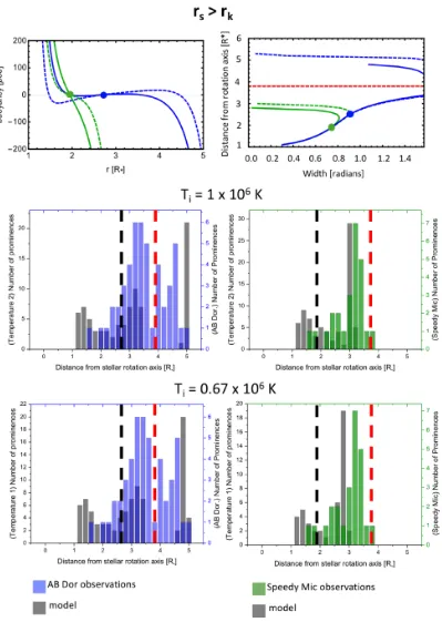
For both stars, a peak is also seen in the model beyond the co-rotation radius and for AB Dor a third peak is seen beyond the source surface at around five stellar radii. The gap seen around 3.5 to 4.5 stellar radii from the rotation axis in the histograms for AB Dor corresponds to the gap seen in the Height-Width curves, denoting a transition from magnetically dominated force balance at low heights, to magneto-centrifugal balance at greater heights. These very tall loops can only be supported when the negative buoyancy of the loop is sufficiently large. This can be seen clearly in the plot of the variation of the buoyancy with height (top left-hand panel). In the case of Speedy Mic, in this parameter range, solutions are not found within the stellar wind since the internal magnetic field strength has fallen to zero before the background field has become open.

Considering now the histograms with a lower internal

temper-ature of Ti= Te/15, the model shows a similar shape of

promi-nence distribution as before but with the peak above co-rotation now shifted to larger heights in both stellar cases. In this parame-ter range, decreasing the temperature causes the top branch of the Height-Width curve to move outwards from the stellar surface. This can be seen most clearly by considering the force balance shown in equation (8). It is worth noting that despite applying the same magnetic fields to both stars, the loops will experience different buoyancy forces due to the difference in gravitational acceleration on the two stars. This leads to different types of behaviours on the two stars.

While tension always acts inwards and the gradient of the external field acts outwards, the direction of the buoyancy force can change.

This term is complicated by the fact that both gand (ρe − ρi)

may take positive or negative values. In the case presented here, the Height-Width curve at low heights does not change significantly with a decrease in internal temperature, due to the dominance of the magnetic field. However, the buoyancy force at large heights becomes larger for a decrease in internal temperature, and since for loops of the same width the tension term will be very similar, this requires a smaller gradient of external field term in order to still reach an equilibrium. This results in the top branch of the curve moving outwards, and thus the final peak in the distribution also moving to larger heights. It should be noted that this behaviour will not always be seen, as it depends on the parameter regime in which we find ourselves, due to the complexity of the buoyancy term.

Speedy Mic. still cannot support prominences within the open field with these parameters, though again the peak of the dis-tribution has shifted outwards. The buoyancy term here is more straightforward since for these parameters the term only changes sign at the co-rotation radius i.e. when the effective gravity changes sign. However, we find ourselves in a similar situation as the buoyancy term acts outwards and becomes larger with decreas-ing temperature, thus once again the peak of the distribution moves outwards.

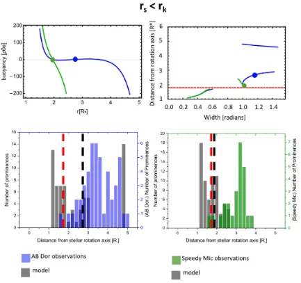
Plotting prominence distributions for a source surfacebelow

co-rotation, with parameters as Fig.7, results in rather different

be-haviour, as shown in Fig.9. For AB Dor the gap in the Height-Width

curve shown in Fig.7can be seen clearly, in addition to another

gap around the source surface. For Speedy Mic however, the rapid rise in the magnitude of the buoyancy above the co-rotation radius cannot be balanced by the loop tension without the added effect of the upwards pressure gradient of the external field. In this case,

Figure 8. Top Panel: Buoyancy (ρe−ρi)/gef(left) and Height-Width plots (right) for AB Doradus (blue) and Speedy Mic (green). The co-rotation radii for the

stars are shown by dots. Middle and Bottom Panels: Histograms of prominence observations for the two stars and example distributions in grey for an internal temperature ofTi=Te/10 andTi=Te/15. The co-rotation radius and source surface (rs=3.8 R) are shown by the black and red dashed lines, respectively.

Parameters here are as Fig.6.

because the field is open above the co-rotation radius, it is im-possible to achieve force balance for heights significantly above co-rotation and so the distribution of model equilibrium heights is extremely compact.

4 D I S C U S S I O N

The effective gravity of a star, and in particular its rotation rate, clearly has a strong influence on the equilibrium summit heights of loops that have cooled. The geometry of the background field may

Figure 9. Top Panel: Buoyancy (left) and Height-Width plots (right) for AB Doradus (blue) and Speedy Mic (green). The co-rotation radii for the stars are shown by dots. Bottom Panel: Histograms of prominence observations for the two stars and example distributions in grey for an internal temperature ofTi=

Te/10. The co-rotation radius and source surface (rs=1.8 R) are shown by the black and red dashed lines, respectively. Parameters here are as Fig.6.

also play a role, however, of particular important is the radius at which this background field becomes open.

4.1 Changing the field topology

With this model we have prescribed both dipolar and quadrupolar stellar fields. These are the two lowest order terms in the multipo-lar expansion for the overall structure of the stelmultipo-lar magnetic field and are the ones most likely to dominate at the large heights at which prominences are observed. The quadrupolar field would nat-urally result in prominences of smaller angular extent. This topology would also be able to explain the presence of four prominences in each hemisphere at one time, as opposed to the two prominences from the dipolar field.

The two multipoles examined here also show slight variation in

the maximum attainable height of these loops, withr=5.98 R

andr=5.34 Rfor the dipole and quadrupole, respectively. This

is explained by the fact that the prescribed quadrupolar magnetic field falls off more rapidly with height than the dipolar field. The difference in maximum height is small, and it is unlikely that from

observed prominence heights alone one would be able to predict the loop topology that best describes the prominence hosting loop. This maximum height is also dependent on the loop parameters, which cannot be obtained directly from observational data.

Although results have only been shown for a dipole and quadrupole external field, in principle any external magnetic field may be prescribed here. This could include higher order multipole expansions, a combination of the multipole expansions, or an en-tirely different external field.

4.2 Inclusion of a source surface

Results here replicate the essential conclusion of Jardine & van

Ballegooijen (2005) that prominences may be supported within the

open field region, i.e. within the stellar wind. We find equilibria for source surfaces both above and below the co-rotation radius, and in both cases ‘helmet streamer’ loop shapes can be found. Solutions around the source surface are, however, difficult to find.

In the case ofrs>rk, the Height-Width curve generated is similar

in form to that of the pure dipole case with an upper and lower

branch, separated by a gap around the location of the source surface. Once the source surface is brought inside of co-rotation, however,

(Fig.7) the family of solutions now shows a middle branch, with

gaps above and below it, although it still retains the same overall shape. Loops in this case have considerably flatter loop summits, in order to balance the forces acting on them, than is seen in the other cases presented here.

The location of the gap in equilibria due to the growth in the buoy-ancy force above co-rotation depends on the loop parameters (such as the temperature and field strength) and the stellar parameters (principally the effective gravity). Its presence could therefore be difficult to detect by compiling a histogram of all observed promi-nences, since they may have a variety of parameters. The gap due to the location of the source surface is at the same height for all loops however.

4.3 Development from previous models

One of the main limitations of Jardine & van Ballegooijen (2005)

was that it was restricted to a Cartesian geometry. It is therefore most suitable for small scales where the star is locally flat. By extending this to a spherical geometry, we have been able to allow for the global field structure of star. In addition, we have removed the infinite horizontal domain implicit in the earlier models. In the

present model, loop footpoints may only extend toπradians in the

dipolar case andπ/2 radians in the quadrupolar case.

As a result of the Cartesian geometry, the solutions of Jardine &

van Ballegooijen (2005) did not allow equilibria at the co-rotation

radius, if this was above the source surface (i.e. in the open field region). The reason is that at the co-rotation radius, the effective gravity, and hence the buoyancy force, is zero. In a Cartesian ge-ometry, however, the field lines in the wind region are straight and purely vertical and so there is no gradient in the magnetic pressure to balance the loop tension. As a result, no equilibria exist. In a spherical geometry, the magnetic pressure gradient does not vanish in the radial field of the wind and so equilibria may still exist at the co-rotation radius.

In principle, the source surface model here does not require a specific prescribed external field, as is the case in the Cartesian model, and various multipoles could be prescribed in the place of the dipole. This model is still restricted to the equatorial plane, through our definition of the effective gravity term, and development of this into a fully three-dimensional model would be interesting but complex.

4.4 Interpreting the observed distributions of prominence heights

The aim of this work is not to attempt to reproduce the observed distributions of prominence heights in detail, but to shed light on their overall structure. The observations reveal the location of large prominences that form at heights of several stellar radii. Smaller, more low-lying prominences (such as those predicted by our mod-els) may be present, but they would not produce sufficiently large absorption signatures to be detected. We therefore focus on the height distributions of the larger prominences that are supported at greater heights.

Our analysis reveals that there may be two gaps in the prominence distribution, caused by two different physical effects. The first is the location of the source surface, where the field transitions from closed to open. This is at a fixed location in our model. The second gap is due to the behaviour of the buoyancy, which for the tallest equilibria

is the dominant force opposing the tension of the cool loop. As can

be seen from Fig. 8, this force behaves quite differently in our

two example stars. For Speedy Mic the co-rotation radius is much closer to the stellar surface, with the result that centrifugal effects dominate at lower heights. This leads to a more compact distribution of equilibria, regardless of the location of the source surface. The buoyancy force depends not only on the effective gravity, which is a global stellar parameter, but also on the local parameters (such as the

temperature) for each cool loop. We show in Fig.8the effect on this

term of a change in the temperature. Although this is less significant than the difference between the two stars, it can still change the location and width of the gap in loop equilibria. Consequently, if a star has cool loops at a range of temperatures, any gaps due to buoyancy effects may be smeared out in the distribution of observed prominence heights.

It should also be noted that the histogram for the observed data for Speedy Mic came from one observing run, with only a few data points, while the data used for AB Dor came from a 10 yr period. The magnetic field structure for AB Dor had changed over this time period (varying by an order of magnitude over 10 yr, corresponding

to a change inβof 0.01) and thus the histogram plotted may in fact

be a combination of multiple histograms. We do not have X-ray data over this extended period and so we do not know if the coronal temperature varied. Extended observations of a star, long enough to include a meaningful number of data points and catch prominences at all heights, taken over a shorter time period than the data used here for AB Dor would be needed in order to better compare the model to data.

5 S U M M A RY A N D C O N C L U S I O N S

We present a model for calculating mechanical equilibrium of mag-netic loops for rapidly rotating stars in a spherical geometry. We model families of solutions for loops embedded in a background field that is either a dipolar or quadrupolar geometry, showing that the model is able to adapt to different stellar magnetic field topolo-gies. We have included the effect of the magnetic field becoming

open beyond some radius (the source surface), both within and

outside of co-rotation, and solutions have been found in the open

field region as in Jardine & van Ballegooijen (2005). Using these

solutions, we show histograms of prominence heights for various prominence temperatures and compare to data from AB Dor and Speedy Mic. The model is able to predict the peak of prominences above the co-rotation radius, but also predicts many prominences at low heights, where they cannot be detected by current methods.

Unlike the Cartesian model previously presented by Jardine &

van Ballegooijen (2005), our spherical geometry allows for

equilib-ria that pass smoothly through the co-rotation radius. This matches the observational data from AB Dor. Looking at the Height-Width curves, we notice that lower solutions are almost force free, fol-lowing the external field very closely, before the buoyancy term becomes important and can no longer be ignored, ultimately deter-mining the maximum height once the force has become too large to be balanced. We find that the exact balancing of these forces is complex, based on the buoyancy force which may act outwards or inwards depending on both the direction of the effective gravity and the sign of the density difference. By comparison of the observed prominence distributions, we expect Speedy Mic to have a more compact corona than AB Dor, since a third peak of prominences is not seen here, which is consistent with the stronger effective gravity force of this star due to its larger radius and shorter rotation period. We note that for both stars the overall shape of the height

tions is closer to that observed when the opening radius is beyond the co-rotation radius.

We have identified two physical processes that can produce gaps in the height distribution of prominences. The first is the opening up of field lines at the source surface and the second is the magnitude and direction in which the buoyancy force acts. This second process will vary from loop to loop if individual loops are at different temperatures and this may act to disguise the presence of this gap in distributions of prominences for an entire star. The location of the source surface may be more robust to variations from loop to loop and so this may be detectable in distributions of observed prominence heights if these are acquired over a short enough time period that the background stellar field does not evolve.

AC K N OW L E D G E M E N T S

The authors would like to thank the referee for helpful comments that improved the paper and acknowledge support from STFC.

R E F E R E N C E S

Aarnio A. N., Matt S. P., Strassun K. G., 2012,ApJ, 760, 1 Altschuler M. D., Newkirk G., 1969,Sol. Phys., 9, 131

Barnes J. R., Cameron A. C., Unruh Y. C., Donati J.-F., Hussain G. A. J., 1998,MNRAS, 299, 904

Barnes J. R., Cameron A. C., James D. J., Donati J.-F., 2000,MNRAS, 314, 162

Byrne P. B., Eibe M. T., Rolleston W. R. J., 1996, A&A, 311, 651 Cameron A. C. et al., 1999,MNRAS, 308, 493

Cameron A. C., 1996, International Astronomical Union. Kluwer Academic Publishers, Dordrecht, p. 449

Cameron A. C., 1999, ASP Conf. Ser., 158, 146 Cameron A. C., Robinson R., 1989,MNRAS, 236, 57 Cameron A. C., Woods J. A., 1992,MNRAS, 258, 360

Cassinelli J. P., Brown J. C., Maheswaran M., Miller N. A., Telfer D. C., 2002,ApJ, 578, 951

Close L. M., Thatte N., Nielsen E. L., Abuter R., Clarke F., Tecza M., 2007,

ApJ, 665, 736

Cranmer S. R., 2017,ApJ, 840, 1

Donati J.-F., Cameron A. C., 1997,MNRAS, 291, 1 Donati J.-F., Landstreet J., 2009,ARAA, 47, 333

Donati J.-F., Cameron A. C., Hussain G. A. J., Semel M., 1999,MNRAS, 302, 437

Dunstone N. J., Barnes J. R., Cameron A. C., Jardine M., 2006a,MNRAS, 365, 530

Dunstone N. J., Cameron A. C., Barnes J. R., Jardine M., 2006b,MNRAS, 373, 1308

Eibe M., 1998, A&A, 337, 757 Ferreira J. M., 2000,MNRAS, 316, 647

Gonzalez W. D., Joselyn J. A., Kamide Y., H. W. Kroehl G. R., Tsuruani B. T., Vasyliunas V. M., 1994,J. Geophys. Res., 99, 5771

Guirado J. C. et al., 2010, ASSSP, Highlights of Spanish Astrophysics V. Springer-Verlag, Berlin Heidelberg,p. 139

Guirado J. C., Marcaide J. M., Marti-Vidal I., Le Bouquin J. B., Close L. M., Cotton W. D., Montalban J., 2011, A&A, 533, A106

Hall J. C., Ramsey L. W., 1992,AJ, 104, 1942

Hall J. C., Huenemoerder D. P., Ramsey L. W., Buzasi D. L., 1990, A&A, 358, 610

Hussain G. A. J. et al., 2005,ApJ, 621, 999

, Hussain G. A. J., 2013, in Brigitte S., Jean-Marie M., S.T Wu, eds, Proc. IAU Symp. 300, Observations of stellar coronae and prominences. Kluwer, Dordrecht, p. 309

Innis J. L., Thompson K., Coates D. W., Lloyd Evans T., 1988,MNRAS, 235, 1411

Jardine M., Cameron A. C., 1991,Sol. Phys., 131, 269 Jardine M., van Ballegooijen A., 2005,MNRAS, 361, 1173 Jardine M., Cameron A. C., Donati J.-F., 2002a,MNRAS, 333, 339 Jardine M., Wood K., Cameron A. C., Donati J.-F., Mackay D. H., 2002b,

MNRAS, 336, 1364

Jeffries R. D., 1993,MNRAS, 262, 369

Khodachenko M. L. et al., 2007,Astrobiol., 7, 167

Leitzinger M., Odert P., Zaqarashvili T. V., Hanslmeier R. G. A., Lammer H., 2016,MNRAS, 463, 965

Low B., 1994,Phys. of Plas., 1, 1684 Low B. C., 2006,ApJ, 646, 1288

Odert P., Leitzinger M., Hanslmeier A., Lammer H., 2017,MNRAS, 472, 876

Owocki S. P., ud-Doula A., Townsend R. H. D., Petit V., Sundqvist J. O., Cohen D. H., 2016,MNRAS, 462, 3830

Parker E. N., 1975,ApJ, 201, 494 Petit V. et al., 2013,MNRAS, 429, 398 Schroder K.-P., 1983, A&A, 124, 16

Skelly M., Unruh Y., Cameron A. C., Barnes J., Donati J.-F., Lawson W., Carter B., 2008,MNRAS, 385, 708

Skelly M. B., Unruh Y. C., Barnes J. R., Lawson W. A., Donati J.-F., Cameron A. C., 2009,MNRAS, 399, 1829

Skelly M. B., Donati J. F., Bouvier J., Grankin K. N., Unruh Y. C., Artemenko S. A., Petrov P., 2010,MNRAS, 403, 159

Spruit H. C., 1981, A&A, 98, 155 Stauffer J. et al., 2017,AJ, 153, 152

Steeghs D., Horne K., Marsh T. R., Donati J. F., 1996,MNRAS, 281, 626 Townsend R. H. D., Owocki S. P., 2005,MNRAS, 357, 251

Ud-Doula A., Owocki S. P., Townsend R. H. D., 2008,MNRAS, 385, 97 Vida K. et al., 2016, A&A, 590, A11

Villarreal D’Angelo C., Jardine M., See V., 2018,MNRAS, 475, L25 Wang J., Zhou G., Zhang J., 2004,ApJ, 615, 1021

This paper has been typeset from a TEX/LA_{TEX file prepared by the author.}