arXiv:1507.05782v1 [math.DS] 21 Jul 2015
THE RANDOM CONTINUED FRACTION TRANSFORMATION
CHARLENE KALLE, TOM KEMPTON, AND EVGENY VERBITSKIY
Abstract. We introduce a random dynamical system related to continued fraction ex-pansions. It uses random combination of the Gauss map and the R´enyi (or backwards) continued fraction map. We explore the continued fraction expansions that this system produces as well as the dynamical properties of the system.
1. Introduction
In 1913 ([Per50]) Perron described an algorithm producing finite and infinite continued fraction expansions of real numbers of the form
x=d0+
ǫ0
d1+
ǫ1
d2+. .. +
ǫn−1
dn+. ..
,
where d0 ∈ Z and for each n ≥ 1, ǫn−1 ∈ {−1,1}, dn ∈ N and dn+ǫn ≥ 1. Moreover, in case the continued fraction is infinite, the algorithm guarantees thatdn+ǫn+1 ≥1 infinitely often. Perron called these expansions semi-regular continued fractions.
Within this framework one can see a number of more familiar systems of continued frac-tions, each of which can be studied by a corresponding dynamical system. Regular con-tinued fractions, which correspond to letting each ǫn = 1, are generated by the Gauss map T x = 1
x (mod 1). Backwards continued fractions, which were introduced by R´enyi in [R´en57], correspond to ǫn = −1. Odd and even continued fractions ([HK02]) and α -continued fractions ([Nak81]) can also be seen within this framework. In this article we define a random dynamical system which allows one to generate all semi-regular contin-ued fraction expansions of the form (1) for any given x and to study their dynamical and ergodic properties. We do not require the condition that dn+ǫn+1 ≥ 1 infinitely often, which makes our set-up slightly more general.
2010Mathematics Subject Classification. Primary: 37C40, 11K50.
Key words and phrases. Continued fractions, random dynamical systems, absolutely continuous invari-ant measures, transfer operator.
Acknowledgements: The first author was supported by the NWO Veni-grant 639.031.140. The second author was supported by EPSRC grant EP/K029061/1.
Over the last decade there has been a great deal of work on random dynamical systems. A random system is given by a finite family of maps defined on the same state space and a probabilistic regime for choosing one of these maps at each time step. The study of condi-tions that guarantee the existence of an invariant measure for such systems was initiated by Morita ([Mor85]) and Pelikan ([Pel84]). They consider the case where each map in the random system is piecewise smooth with respect to some finite partition and expanding on average. In [GB03] and [BG05] these results are extended to when the probabilistic regime is position dependent. These results were further generalised by Inoue ([Ino12]) to more general underlying partitions, including ones with countably many elements. In [ANV] limit theorems are studied for random systems consisting of countably many maps. Their examples include families of maps that are piecewise smooth with respect to some finite partition and are expanding on average. Rousseau and Todd studied hitting time statistics for random maps [RT15].
Random dynamical systems have also been used in relation to representations of numbers, see for example [Mor]. In particular, the introduction of the random β-transformation has opened up new approaches to studying the dynamical and ergodic properties of β -expansions and Bernoulli convolutions, see [DdV05, DK13, Kem13]. A key part of this approach was to study the invariant measures and ergodic properties of the random β -transformation, as was done in [DdV05, DdV07, Kem14].
In this article we first introduce the random continued fraction map K. We show that it generates convergent continued fraction expansions for all points in its domain and we explore some of the properties of these expansions. The map K, and a related map R
which is easier to analyse, present several challenges which are interesting from a purely dynamical point of view. In particular, R has countably many discontinuities and one of the interval maps definingRhas an indifferent fixed point. To overcome these difficultieswe build on the work of Inoue [Ino12], who studied transfer operators for countably branched skew product systems that are expanding on average. We can then use the results from [ANV] to obtain limit theorems. Other specific examples of random intermittent systems have been recently considered in [BBD14]. Here Bahsoun, Bose and Duan studied limit theorems and mixing rates for random combinations of maps that are variations of the Manneville-Pomeau map.
fact is quite smooth. In the last section we discuss this in more detail and also mention some open questions and future directions.
2. The random map
2.1. Definition of the map. It is clear that x∈R has an expansion of the form
(1) x= ǫ0
d1+
ǫ1
d2+. .. +
ǫn−1
dn+. ..
,
where ǫn−1 ∈ {−1,1}, dn∈N and dn+ǫn≥1 for all n ∈N if and only if x∈[−1,1]\{0}. If |x| > 1, we can subtract a suitable integer d0 from x and use the representation from (1) for x−d0 to obtain a continued fraction expansion of x.
To find the right definition of the random dynamical system K, we first ask which x ∈
[−1,1] have expansions that begin with a given choice of ǫ0 and d1. Let ǫ0 and d1 > 1 be given. Then x can be written in the form (1) if and only if x = ǫ0
d1+y for some y ∈
[−1,1]\ {0}. This can be satisfied if and only if ǫ0 =sgn(x) and
|x|=ǫ0x∈
1
d1+ 1
, 1 d1−1
.
This typically gives two choices of the digit d1. We see that
y= ǫ0
x −d1 =
1 |x| −d1.
Similarly, if d1 = 1 then we require ǫ1 = 1 and have x= d1ǫ+y0 for somey ∈(0,1]. This can be satisfied for |x| ∈(12,1] and we have
y= 1 |x| −1.
As is standard with dynamical constructions of expansions of real numbers, the possible values of ǫ1, d2 are equal to the values of ǫ0, d1 associated with y = |1x|−d1. Thus we can generate all expansions of the form (1) using the following transformation.
Let Ω = {(ωk)k≥1 : ωk ∈ {0,1}} = {0,1}N and let σ : Ω → Ω be the left shift. We define the random continued fraction map K : Ω × [−1,1] → Ω × [−1,1] by setting
K(ω,0) = (σ(ω),0) and for |x| ∈ k+11 ,k1,
K(ω, x) =σ(ω),1 x
−(k+ω1)
-1 -1
2 -13--1415 0 151413 12 1
1
[image:4.612.211.391.100.296.2]0
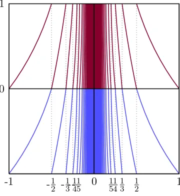
Figure 1. The map T0 in red and T1 in blue.
One can think of the map K as follows. Let maps T0, T1 : [0,1]→[0,1] be the Gauss and R´enyi maps respectively, given by
(2) T0x=
0, if x= 0,
1
x (mod 1), otherwise,
and T1x=
0, if x= 1,
1
1−x (mod 1), otherwise.
Let π: Ω×[−1,1]→[−1,1] be given by π(ω, x) =x. Then
π K(ω, x)=
T0x−ω1, if x >0,
T1(x+ 1)−ω1, if x <0.
Set ω0 = 0 if x≥0 and 1 otherwise. This gives
(3) π K(ω, x)=Tω0(x+ω0)−ω1.
Note that π K(ω, x) ∈ [0,1] if ω1 = 0 and π K(ω, x)
∈ [−1,0] if ω1 = 1. By iterating we see that for each n ≥ 1 and all (ω, x) ∈ Ω×[−1,1], such that π Km(ω, x) 6= 0 for 0≤m < n, we have
π Kn(ω, x)= (Tωn−1 ◦ · · · ◦Tω0)(x+ω0)−ωn.
2.2. Random continued fraction expansions. Forn = 1, set
d1 =d1(ω, x) =
k+ω1, if |x| ∈
1 k+1,
1 k
i
,
and for n ≥2, define dn(ω, x) =d1 Kn−1(ω, x)
. We have
(4) π K(ω, x)= (−1)ω01
x −d1.
and for eachn ≥1 such thatπ(Km(ω, x))6= 0 for all 0≤m≤n,
x= (−1) ω0
d1+π(K(ω, x))
= (−1) ω0
d1+
(−1)ω1
d2+π(K(ω, x))
=· · ·= (−1) ω0
d1+
(−1)ω1
d2+. .. +
(−1)ωn−1 dn+π(Kn(ω, x))
.
The digit sequence dn(ω, x)
n≥1 represents the continued fraction representation of the pair (ω, x) as given by K. If there is a smallest integer n such that dn(ω, x) = ∞, then (ω, x) has finite random continued fraction expansion
x= (−1) ω0
d1+
(−1)ω1
d2+. .. + (− 1)ωn−2 dn−1
.
Now suppose thatdn(ω, x) is finite for alln ≥1. We want to show that (ω, x) has infinite
random continued fraction expansion
x= (−1) ω0
d1+
(−1)ω1
d2+. .. + (− 1)ωn−1
dn+. ..
.
For each n ≥1, let pn
qn denote the convergents of the random continued fraction of (ω, x),
i.e., write
pn
qn
= (−1)
ω0
d1+
(−1)ω1
d2+. .. + (− 1)ωn−1
dn
.
2.3. Convergence of Partial Sums. To show convergence, we follow the approach for regular continued fractions with the important difference that in our case the numbers qn do not necessarily increase. As for regular continued fractions (see for example [DK02]), one can obtain the following relations:
p−1 = 1, p0 = 0, pn=dnpn−1+ (−1)ωn−1p
n−2,
q−1 = 0, q0 = 1, qn=dnqn−1+ (−1)ωn−1q
Using these recurrences, induction easily gives that
(5) x= pn+pn−1π K
n(ω, x)
qn+qn−1π Kn(ω, x)
and that
(6) pn−1qn−pnqn−1 = (−1)n(−1)ω0+···+ωn−1.
The next lemmas are needed to show that although the sequence{qn}n≥1 is not necessarily increasing, we still have limn→∞ q1n = 0.
Lemma 2.1. For each n ≥ 2, qn > 0 and if qn ≤ qn−1, then ωn−1 = 1 and dn = 1, so
ωn= 0.
Proof. We prove this by induction. For n = 1 we have q1 =d1 ≥ 1 = q0. For n = 2, we have q2 =d2d1+ (−1)ω1 and hence
q2 ≤q1 ⇔ d2 ≤1−
(−1)ω1
d1
.
This can happen only if ω1 = 1, thus d1 >1, and d2 = 1. This gives q2 =d1 −1>0 and the lemma. Now suppose the statements hold for all k < n, i.e., qk > 0 and if qk ≤ qk−1, thenωk−1 = 1 anddk= 1, so ωk= 0. If qn > qn−1, then automaticallyqn >0. So, suppose
qn≤qn−1. We have
qn=dnqn−1+ (−1)ωn−1q
n−2 ≤qn−1 ⇔ 1≤dn≤1−(−1)ωn−1qn−2 qn−1
.
Since qn−2, qn−1 >0, qn ≤qn−1 implies that ωn−1 = 1 and hence dn−1 >1. The induction hypothesis then gives that qn−2
qn−1
<1 and hence 1≤dn<2. This gives the lemma.
Lemma 2.2. If qn ≤qn−1, then qn−2 < qn−1 < qn+1. This implies that qn 6=qn−1.
Proof. By the previous lemma we have ωn−1 = 1, so qn−1 > qn−2. We also have dn = 1 and thus ωn = 0. Since qn > 0, this implies that qn+1 = dn+1qn +qn−1 > qn−1. For the second part, note that ifqn=qn−1, then dn= 1−(−1)ωn−1qn−2
qn−1
and by the previous lemma
qn−1 > qn−2. Since dn is an integer, this is not possible.
Before we can prove that the process converges, we need a lower bound on the qn’s in case
qn< qn−1. This is done in the next lemma.
Lemma 2.3. Suppose qn< qn−1, so dn−1 >1.
(i) If dn−1 >2, then qn> qn−2.
(ii) If dn−1 = 2 and (ωk, dk) = (1,2)for all 1≤k ≤n−1, then qn = 1 and qn−1 =n. (iii) Supposedn−1 = 2 and there is a 1≤k < n−1 such that (ωk, dk)6= (1,2). Let k be
Proof. Recall that qn < qn−1 implies that dn = 1, ωn = 0 and ωn−1 = 1, so dn−1 > 1. Hence, qn=qn−1−qn−2.
(i) If dn−1 >2, then
qn = dn−1qn−2+ (−1)ωn−2q
n−3−qn−2 = (dn−1−1)qn−2+ (−1)ωn−2q
n−3
≥ 2qn−2+ (−1)ωn−2q
n−3.
If qn−2 > qn−3, then qn≥ 2qn−2−qn−3 > qn−2. If qn−2 < qn−3, then Lemma 2.1 gives that
ωn−2 = 0 and hence qn≥2qn−2+qn−3 > qn−3 > qn−2.
For both (ii) and (iii), note that if dk = 2 and ωk = 1 for some 1 ≤ k ≤ n −1, then
qk = 2qk−1−qk−2, so
(7) qk−qk−1 =qk−1−qk−2. (ii) From (7) it follows that
qn =qn−1−qn−2 =q2−q1 = 2·2 + (−1)1−2 = 1. Moreover, for each 1≤k ≤n−1 it holds that
qk = 2qk−1−qk−2 =qk−1+ (qk−1−qk−2) =qk−1+ 1.
Hence, qn−1 =n−2 +q1 =n.
(iii) Let k be as given in the lemma, so (ωk, dk) 6= (1,2) and (ωj, dj) = (1,2) for k+ 1 ≤
j ≤n−1. Then,
qn =qn−1−qn−2 =qk+1−qk =dk+1qk+ (−1)ωkqk−1−qk =qk+ (−1)ωkqk−1.
Ifωk = 0, thenqn=qk+qk−1 > qk−1. If ωk= 1, thendk≥3 and qk> qk−1 by Lemma 2.1. This gives
qn =qk−qk−1 = (dk−1)qk−1+ (−1)ωk−1q
k−2 ≥2qk−1+ (−1)ωk−1q
k−2.
As in the proof of part (i) we now get that ifqk−1 > qk−2, thenqn > qk−1 and ifqk−1 < qk−2, then ωk−1 = 0 and we also get qn > qk−1.
Proposition 2.1. Let x ∈ [−1,1]\Q. For each ω, the digits dn(ω, x) give a continued
fraction expansion of x.
Proof. For alln ≥1 we have using (5) and (6)
x− pn
qn
=
qn pn+pn−1π Kn(ω, x)
−pn qn+qn−1π Kn(ω, x)
qn qn+qn−1π Kn(ω, x)
=
π Kn(ω, x)(qnpn−1 −pnqn−1)
qn qn+qn−1π Kn(ω, x)
≤ 1
|qn qn+qn−1π Kn(ω, x)
| ≤
1
qn|qn−qn−1| ≤ 1
qn
.
We now show that limn→∞q1n = 0. Let ε > 0. By Lemma 2.2 there exists a subsequence
(qnk)k≥0 such that limk→∞
1
qnk = 0 and hence there exists an N1 such that 1
is non > N1, such thatqn< qn−1, then we are done. If there is, let k be the smallest such index. If (ωN1+1, dN1+1)6= (1,2), by Lemma 2.3 qk ≥qN1 and then same holds for all other
n > N1. If (ωN1+1, dN1+1) = (1,2), then set N =k+ 1. We then have
1 qN <
1 qk−1
< q1
N1 < ε.
Moreover, for all n > N we have qn > qk−1, since (ωk, dk) = (0,1). This shows that the limit exists and is equal to 0. Hence we get
x= (−1) ω0
d1+
(−1)ω1
d2+
(−1)ω2
d3+. ..
for each x∈[−1,1]\Q.
3. Invariant densities
Recall that T0, T1 : [0,1] → [0,1] are the Gauss and R´enyi map respectively. To study the dynamical properties of random continued fractions we replace the map K by the transformation R: Ω×[0,1]→Ω×[0,1] given by
R(ω, x) = (σω, Tω1x).
The ergodic properties of R are easier to study and (3) gives the following simple relation between K and R. Recall thatω0 = 0 if x≥0 and 1 otherwise. Then,
π Rn−1(ω, T0x)
=π Kn(ω, x)+ωn,
and hence,
π Kn(ω, x)=ωn+ (−1)ωnπ Rn−1(ω, T0x)
.
Using this we can recover the digit sequence dn(ω, x)
n≥1 generated by K as follows. For (ω, x)∈Ω×[0,1] define
(8) b(ω, x) =
k+ω2, if ω1+ (−1)ω1x∈ k+11 ,1k
,
∞, if ω1+ (−1)ω1x= 0. Write 0ω for the sequence ω′ ∈Ω satisfyingω′
1 = 0 andωn+1′ =ωn for all n≥1. Then for
n≥1,
(9) dn(ω, x) =b Rn−1(0ω, x)
.
Remark 3.1. The Gauss mapT0 is intimately related to the well known Farey map, which is defined by
F x=
x
1−x, if 0≤x≤
1 2,
1−x x , if
1
The Gauss map can be obtained from F by inducing on the first passage time to the interval 1
2,1
. For x ∈ [0,1] and n ≥ 1, set ωn = 1 if π Rn−1(ω, x)
< 12 and ωn = 0 if
π Rn−1(ω, x) > 12. If π Rn−1(ω, x) = 1
2, you can choose. Then π R
n(ω, x) = Fnx for
each n ≥1.
3.1. Existence. Let λ denote the Lebesgue measure on [0,1]. We are going to show that
R has invariant measures of type mp⊗µp, where mp is the (p,1−p)-Bernoulli measure on Ω and µp is a probability measure on [0,1] absolutely continuous with respect to λ. For this we use [Ino12]. Recall that a function g : [0,1] → [0,1] is said to have bounded variation if
_
[0,1]
g := sup
0=x0<x1<x2<···<xn=1
n
X
i=1
|g(xi)−g(xi−1)|<∞.
The following is a very simplified, discrete version of the main theorem of [Ino12]:
Theorem 3.1 (Inoue, [Ino12]). Given two non-singular maps T0, T1 : [0,1] → [0,1], let
R :{0,1}N×[0,1]→ {0,1}N×[0,1] be given by
R(ω, x) = (σ(ω), Tω1(x)).
Letp∈[0,1]and set p0 =pandp1 = 1−p. Fori∈ {0,1}let {Ii,k}be a countable partition
of [0,1] into intervals and use int(Ii,k) to denote the interior of these intervals. Let g(i, x)
be functions satisfying
(10) g(i, x) = pi
|T′
i(x)|
on Skint(Ii,k). Assume that the following conditions are satisfied:
(I1) The restrictions of Ti to each interval int(Ii,k) are C1 and monotone. (I2) The weighted average expansion of Ti is uniformly positive for all x, i.e.,
sup x∈[0,1]
g(0, x) +g(1, x)<1.
(I3) For each i∈ {0,1} the functions g(i, x) : [0,1]→R are of bounded variation.
Then there exists a probability measure µp on [0,1] absolutely continuous with respect to
the Lebesgue measure λ with density function hp that is of bounded variation. Moreover,
µp has the property that
µp(A) =pµp(T0−1A) + (1−p)µp(T1−1A)
for each Borel measurable set A⊆[0,1].
We have not included condition (A2) of Inoue since this automatically holds when one only has a finite number of maps Ti. We apply Theorem 3.1 to our setting.
Proposition 3.1. Suppose p ∈ (0,1). Then the maps T0 and T1 satisfy the conditions
Proof. Fork ≥1, letI0,k = k+11 ,1k
andI1,k =
k−1
k , k k+1
. Consider the following partitions of [0,1]:
(11) I0 ={I0,k}k≥1 and I1 ={I1,k}k≥1.
ThenT0andT1are bothC1and monotone on the interiors of the intervals of their respective partitions, so condition (I1) is satisfied. Note that the functions g(i,·) from (10) become
g(0, x) =px2 and g(1, x) = (1−p)(1−x)2. almost everywhere. We see that
sup x∈[0,1]
g(0, x) +g(1, x)= sup x∈[0,1]
x2−2(1−p)x+ (1−p)= max{1−p, p}.
So condition (I2) is satisfied for all p ∈(0,1). Since both g(0,·) and g(1,·) are monotone functions on the interval [0,1], we have
_
[0,1]
g(0,·) =p and _ [0,1]
g(1,·) = 1−p.
This gives (I3), and the proof
The conclusions of Theorem 3.1 yield the following result, the proof of which is standard, but included for the convenience of the reader.
Theorem 3.2. For any choice of parameter 0< p < 1, there is an absolutely continuous probability measureµp ≪λ such that the product measuremp⊗µp is invariant forR. The
probability density function hp of the measure µp is of bounded variation.
Proof. Theorem 3.1 gives an absolutely continuous measure µp with the property that for each Borel set A⊂[0,1], we have
(12) µp(A) =pµp(T0−1A) + (1−p)µp(T1−1A). Take a cylinder [j1· · ·jn]∈ {0,1}N and an interval (a, b)⊂[0,1]. Then
R−1 [j1· · ·jn]×(a, b)
= [0j1· · ·jn]×T0−1 (a, b)
∪[1j1· · ·jn]×T1−1 (a, b)
.
Hence,
(mp⊗µp)
R−1 [j1· · ·jn]×(a, b)
=p mp([j1· · ·jn])µp
T0−1 (a, b)+ (1−p)mp([j1· · ·jn])µp
T1−1 (a, b)
=mp([j1· · ·jn])µp (a, b)
= (mp⊗µp) [j1· · ·jn]×(a, b)
.
This gives the first part of the result. The density hp is given by Theorem 3.1.
measure with density h0(x) = x1. This was proved by R´enyi in [R´en57]. The fact that R is expanding on average causes thathp is a probability density for all 0< p <1. It would be interesting to analyse the behaviour of hp asp→0.
3.2. Properties of the invariant measure. In this section we list some of the properties of the invariant measure mp ⊗µp. In [Ino12] Inoue proved the existence of the density
hp by analysing a random version of the Perron-Frobenius operator. In our case, the corresponding operatorLp :L1(λ)→L1(λ) is given by
(13) (Lpf)(x) =
X
k≥1
h p
(k+x)2f
1
k+x
+ 1−p (k+x)2f
1− 1
k+x
i
.
Theorem 3.1 is proved in [Ino12] by showing that this operator has a fixed point in the space of functions of bounded variation, which is our function hp. Recall that functions of bounded variation can be modified on a countable number of points to obtain a lower semi-continuous function. From now on we assume thathpis lower semi-continuous. Under the conditions of Theorem 3.1 the operator Lp is quasi-compact and constrictive. In this section we use these results to derive some dynamical properties ofR. We first prove that
R satisfies a strong Random Covering Property.
Proposition 3.2. Let I ⊆[0,1] be a non-trivial interval. Then for every ω ∈Ω, there is an n ≥1 such that
Tωn◦ · · · ◦Tω1
I = [0,1).
Proof. Recall the definition of the partitions I0 and I1 in the proof of Proposition 3.1. If a non-trivial interval J is contained in one of the intervals in Ii, then TiJ is again an interval andλ(TiJ)> λ(J). Hence, there is anm ≥1, such that Tωm◦ · · ·◦Tω1
I contains an endpoint of one of the intervals in Iωm+1. This means that Tωm+1 ◦Tωm◦ · · · ◦Tω1
I
contains an interval of the form [0, c) and an interval of the form (1−c,1) for some c >0. Thus Tωm+2◦ · · · ◦Tω1
I = [0,1).
It now follows that the measureµp is in fact equivalent toλ. The proof below is essentially the one from [ANV].
Proposition 3.3. Let hp be the probability density function from Theorem 3.2. Then
hp(x)>0 for all x∈[0,1).
Proof. We know thathpis a function of bounded variation satisfyinghp ≥0,
R
that hp ≥α1I. Fix a sequence ¯ω = (¯ω1,ω¯2, . . .)∈Ω. Then for any n ≥1,
hp(x) = Lnphp(x) ≥ αLnp1I(x)
= X
(ω1,...,ωn)∈Ωn
X
y∈(Tωn◦···◦Tω1)−1{x}
pω1· · ·pωn
|(Tωn ◦ · · · ◦Tω1)′y|
1I(y)
≥ X
y∈(Tωn¯ ◦···◦Tω¯1)− 1
{x}
p¯ω1· · ·pω¯n
|(Tω¯n◦ · · · ◦Tω¯1)′y|
1I(y).
By Proposition 3.2 there is an n ≥1 such that for allx∈[0,1),
(Tω¯n◦ · · · ◦Tω¯n)−
1{x} ∩I 6=∅.
Hence, for all 0< p <1 and all x∈[0,1),hp(x)>0.
This proposition leads to the following result, the proof of which uses a standard technique that can be found for example in [BG97].
Proposition 3.4. The probability measure hp is bounded from above and away from 0.
Proof. The fact thathp is bounded from above follows since hp is of bounded variation. In the previous proposition, we have established that hp(x)>0 for all x∈[0,1). Sincehp is lower semi-continuous, it takes its minimum on [0,1]. Therefore, it is enough to show that
hp(1) >0. Let ε > 0 be small and let k≥ 1. We consider part of the inverse image of the interval (1−ε,1) under T0 (we could just as well use T1). Note that
1
k+ 1, 1
k+ 1−ε
⊆T0−1(1−ε,1)
and that
λ 1 k+ 1,
1
k+ 1−ε
= ε
(k+ 1)(k+ 1−ε). Hence,
k2λ 1 k+ 1,
1
k+ 1−ε
< λ (1−ε,1)<(k+ 1)2λ 1 k+ 1,
1
k+ 1−ε
.
It then follows that
lim
x↑1hp(x) = limε→0
1
λ (1−ε,1)
Z 1
1−ε
hp(x)dx = lim ε→0
µp (1−ε,1)
λ (1−ε,1)
≥ lim ε→0
pµp T0−1(1−ε,1)
+ (1−p)µp T1−1(1−ε,1)
(k+ 1)2λ 1 k+1,
1 k+1−ε
≥ lim ε→0
pµp k+11 ,k+11−ε
(k+ 1)2λ 1 k+1,
1 k+1−ε
=
p
(k+ 1)2hp
1
k+ 1
>0.
The fact thathp is bounded from above follows sincehp is a function of bounded variation
The fact that the operatorLp is quasi-compact on the set of functions of bounded variation allows us to obtain a number of consequences from the Ionescu-Tulcea and Marinescu Theorem, as is done in many similar situations. The reader is referred to [Bal00] for example for an outline of this approach for deterministic maps. The spectral decomposition (which is already given in [Ino12]) together with Proposition 3.4 gives that 1 is a simple eigenvalue for Lp, that there are no other eigenvalues on the unit circle and that Lnpf →
R
f dλhp in
L1(λ). This means that the system Rsatisfies the conditions of [ANV]. (Note thatRis not contained in the class of random Lasota-Yorke systems discussed in Example 2.1 of [ANV], since both T0 and T1 have infinitely many branches.) From [ANV] we then immediately get exponential decay of correlations:
Proposition 3.5 (see [ANV] Proposition 3.1). There exist constants C ≥ 0 and ρ < 1, such that for all functions f of bounded variation and all g ∈L∞(λ),
Z
[0,1]L n
pf·gdµp−
Z
[0,1]
f dµp
Z
[0,1]
gdµp
≤CρnkfkBVkgk∞.
In particular, R is mixing. A proof can be found in [Mor85] for example.
Theorem 3.3. The random transformation R is mixing with respect to mp⊗µp.
Proof. Define the function φ : Ω×[0,1] → [0,1] by φ(ω, x) = ω1 + (−1)ω1x. Define the cylinder sets of order 1 by
[d]×∆(a)j = [d]×φ
[d]×a 1 + 1,
1
a
i
.
In general the cylinders of order k are given by [d1· · ·dk]×∆(a1, . . . , ak)d1···dk, where
∆(a1, . . . , ak)d1···dk =
k
\
j=1
Tdj−1 ◦ · · · ◦Td1
−1
φ[dj]×
1
aj + 1
, 1 aj
i
.
Write [ ¯d]×∆(¯a)k ¯
d for [d1· · ·dk]×∆(a1, . . . , ak)d1···dk. These sets form a generating
semi-algebra for the σ-algebra on Ω×[0,1]. A straightforward computation using the previous proposition now gives that for any two such cylinders [ ¯d]×∆(¯a)k
¯
d and [¯c]×∆(¯b) ℓ ¯ c,
lim
n→∞(mp⊗µp) R
−n [¯c]×∆(¯b)ℓ ¯ c
∩ [ ¯d]×∆(¯a)kd¯
= (mp ⊗µp) [¯c]×∆(¯b)ℓc¯
(mp⊗µp) [ ¯d]×∆(¯a)kd¯
,
where the convergence is in L1.
by Xk(ω, x) = φ (Tωk ◦ · · · ◦Tω1)x
and Sn = Pnk=0−1Xk. The asymptotic variance σ2 is defined by
σ2 = lim n→∞
1
n
Z
Ω×[0,1]
Sn2d(mp⊗µp).
In [ANV] it is proved that this limit exists in Proposition 3.2. Let M be the set of all Borel probability measures on [0,1] that are absolutely continuous w.r.t. λ with a density of bounded variation.
Theorem 3.4 (Central Limit Theorem, see [ANV] Theorem 3.5). Let ν ∈ M. Then the process √Sn
n
n≥1 converges in law to N(0, σ
2) under the probability measure m p ⊗ν.
Theorem 3.5(Large Deviation Principle, see [ANV] Theorem 3.6). Supposeσ2 >0. Then
there exists a non-negative rate function c, continuous, strictly convex, vanishing only at 0, such that for every ν ∈ M and every sufficiently small ε >0,
lim n→∞
1
nlog (mp⊗ν)(Sn> nε)
=−c(ε).
In particular these results hold forλ and µp.
4. Further Properties of the continued fractions
Here we make a few observations about the continued fractions produced by K.
4.1. Counting Expansions. It is clear that K produces all semi-regular continued frac-tions of points x ∈ [−1,1]. Since typically each sequence ω ∈ Ω characterises a unique continued fraction expansion, K will generate uncountably many different continued frac-tion expansions for most x.
Proposition 4.1. Each x∈[−1,1]\Q has uncountably many different continued fraction expansions given by K. Each x∈([−1,1]∩Q)\{0} has countably infinitely many.
Proof. To prove this we first show thatx∈([−1,1]∩Q)\{0}if and only if for each ω ∈Ω there exists an n ≥ 0 such that π Kn(ω, x) ∈ 1k,−1k : k ∈ N . One direction is clear, since if x is irrational then π(K(ω, x)) is irrational for any ω ∈ Ω. Now assume that
x ∈ [−1,1]∩Q\{0}. First note thatπ K(ω, x) ∈ {−1,0,1} if and only if x ∈ 1k,−1k :
k ≥1 . Write x = r1
r0 with r0, r1 ∈Z and |r1| ≤ |r0|. If |r0|=|r1|, then the proposition is
obtained with n = 0. If not, then
π K(ω, x)= (−1) ω0
x −d1 =
(−1)ω0r
0−r1d1
r1
= r2
r1 ∈
[−1,1].
Herer2 ∈Z and |r2| ≤ |r1|. If |r2|=|r1|, then we have the proposition with n = 0. If not, then by continuing in the same manner we obtain a sequence of integersr0, r1, . . . , rnwith
Now supposex∈[−1,1]\Q. Then there is noω∈Ω and non≥0, such thatπ Kn(ω, x) ∈
±1
k : k ≥1 . Hence, eachω produces a unique continued fraction expansion forx. This gives the first part of the proposition.
For the second part of the statement, let pq be an arbitrary element of ([−1,1]∩Q)\{0} with p ∈ Z, q ∈ N and 0 < |p| < q. Then for each ω ∈ Ω there is an N ≤ q, such that
π KN(ω,pq)∈1k,−1k . If ωn = 1 for alln > N, then there is some k ≥1 such that
dn ω,p q
n≥1 = (d1, . . . , dN, k+ 1,2,2,2, . . .). If there is a smallest integer M ≥2 such thatωN+M = 0, then
dn ω,p q
n≥1 = (d1, . . . , dN, k+ 1, 2| {z }, . . . ,2
M−1 times
,1).
Finally, if ωN+1= 0, then
dn ω,p q
n≥1 = (d1, . . . , dN, k).
Hence, K generates only countably many different expansions for x.
Proposition 4.1 gives all the possible endings of digit sequences of rational points pq gen-erated by K. From Figure 1 it is clear however that pq also has expansions that are not generated by K. The corresponding digit sequences are
(d1, . . . , dN, k−1,1), (d1, . . . , dN, k−1,2,2,2, . . .), and for eachM ≥2,
(d1, . . . , dN, k−1, 2, . . . ,2
| {z }
M−1 times
,1).
The fact that K does not generate these expansions is a consequence of having defined K
by taking the intervals k+11 ,1k left-open and right-closed. So all points in [−1,1]∩Q have expansions of the form (1) that are not generated by K, but we know exactly what the missing expansions are.
α-continued fractions. Theα-continued fraction transformation was first introduced by Nakada in [Nak81]. Givenα∈[0,1], define the mapTα : [α−1, α)→[α−1, α) byTα0 = 0 and
Tαx=
1 x − j 1 x
−(α−1) k
for x6= 0. First note that for x <0, T1(1 +x) =
x1− ⌊1x⌋. Also note that
1 x − j 1 x k
< α ⇔ j1 x
−α+ 1 k
=j1
x k and 1 x − j 1 x k
≥α ⇔ j1 x
−α+ 1 k
=j1
x
k
We can define a sequence ω = (ωn)n≥1 ∈ Ω such that for each n ≥0, π Kn(ω, x)
=Tn αx as follows. Note that if 0< x < α, then either T0x∈[α−1, α) in which case we set ω1 = 0 or T0x−1∈[α−1, α), in which case we set ω1 = 1. Similarly forα−1≤x <0 and the map T1(x+ 1). Then
Tω0(x+ω0)−ω1 =Tαx.
We can apply the same procedure for every n ≥ 2 with the point (Tωn−1 ◦ · · · ◦Tω0)(x+ ω0)−ωn. One can easily show, using (3) and induction, that for each x ∈[α−1, α) and
n≥1, one gets π Kn(ω, x)=Tn αx.
4.2. Restrictions on digits. For regular continued fractions, expansions with restrictions on the digits have been thoroughly investigated. Continued fractions with bounded digits have applications in many fields, ranging from formal language theory to diophantine approximation to pseudo-random number generators, see [Sha92] for a survey on this topic. For random continued fractions the following is easily observed.
Proposition 4.2. LetΛ⊂Nbe such that it does not miss two or more consecutive integers, i.e., if k 6∈Λ, then k−1, k+ 1∈Λ. Then all numbers in [−1,1] have a continued fraction expansion of the form (1) with dn∈Λ for each n.
Proof. From Figure 1 it is clear that if we delete the branches 1
x−k and − 1
x−k for k∈Λ, then all the other branches still cover all of the interval [−1,1]. This means that for each
x∈[−1,1] we can choose an ω ∈Ω such that dn(ω, x)6=k for all n≥1.
From this proposition it follows immediately that each x∈[−1,1] has a continued fraction expansion with only even or only odd digits. Moreover, note that if we remove all branches corresponding to the odd (or even) digits, then there is no overlap in the system except on the points ±k1, implying that each irrational x∈[−1,1] has a unique expansion with only odd (or even) digits.
Regular continued fractions with bounded digits are very well studied. It has been known since the works of Jarnik ([Jar32]) and Good ([Goo41]) that for each N ≥ 2 the set of points x∈[0,1] that has a regular continued fraction expansion with digits not exceeding
N has Hausdorff dimension strictly between 0 and 1. Many people have given estimates for the Hausdorff dimension of the set E1,2 of points with a regular continued fraction expansion using only digits 1 and 2, with the most recent result by Pollicott and Jenkinson ([JP01]) calculated the first 25 digits of the Hausdorff dimension of this set:
dimH(E1,2) = 0.5312805062772051416244686. . . .
In the random case we have the following.
Proposition 4.3. The set of points x ∈ [−1,1] that have a continued fraction expansion of the form (1) with dn∈ {1,2} for alln ≥1, has positive Lebesgue measure. In fact, it is
Proof. Let A1,2 denote the set of points that have an expansion of the form (1) with only digits 1 and 2. Then A1,2 ∩ − 13,13
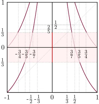
= ∅. First note that the points ±1k, k = 2,3, have countably many expansions using only 1 and 2 as discussed after the proof of Proposition 4.1. These expansions are not generated by K. For all other points in A1,2 such expansions are generated by K. We consider these expansions, see Figure 2 for an illustration.
The first digit of any x∈A1,2∩ 13,12
∪−1 2,−
1 3
must be 2, coming from ω1 = 0. For
n≥1, let Sn denote the map Snx=
1
x
−n. Then for points in the set
E = [ n≥1
S2−n0,1
3
∩1 3,
1 2
i
∪h− 1 2,−
1 3
K does not generate an expansion with only digits 1 and 2. Note that S2 has fixed point
√
2−1 and |S′
2x|>1 for all x∈ 13, 1 2
∪− 1 2,−
1 3
. Since √
2−16∈S2−1h0,1
3
=3 7,
1 2
i
∪h− 1 2,−
3 7
and
S2−2h0,1
3
=h2 5,
7 17
∪− 177 ,2
5
i
,
it follows that E ⊆ 25,12∪− 12,−25 and that E is a countable union of intervals. For the set 12,1∩−1,−12 we have the following. Since
S1−1h0,1
3
=3 4,1
i
∪h−1,−3
4
and S2−1− 1
3,0
i
=h1 2,
3 5
∪− 35,−1
2
i
we see that on 3 4,1
and −1,−34 we will have to use S2 and on 12,35
and − 3 5,−
1 2
we will have to use S1. Note that
S1−1E∩1
2,1
i
⊆h2 3,
5 7
i
.
Since 35 < 23 < 57 < 43, on all of the interval 12,1 we can avoid being mapped into E by making appropriate choices between S1 and S2. Hence
A1,2 =
h1
3,1
i
∪h−1,−1
3
i
\E.
In 1994 Lehner ([Leh94]) proved that every irrational number x in the interval [1,2) has a unique continued fraction expansion of the form
x=b0+
ǫ0
b1 +
ǫ1
b2+. ..
,
-1 -1
2 -13 0 13 12 1
1
1 3
0
-13
-34-35 -37 37 35 34
2 5
[image:18.612.222.384.100.270.2]1 2
Figure 2. Points that have a continued fraction expansion generated byK
with only digits 1 and 2 only use the maps x7→1
x
−1 and x7→1
x
−2.
withb0 = 0. Moreover, there are points that have more than 1 such expansions. This holds for example for all points in the interval 35,23 or in the interval 57,34.
In spite of the result from Proposition 4.3, we have the following results on the asymptotic geometric and arithmetic mean of the digits, which are similar for the regular continued fractions.
Proposition 4.4. For (mp⊗µp)-a.e. (ω, x)∈Ω×[0,1], we have
1< lim
n→∞ d1(ω, x)· · ·dn(ω, x)
1/n
<∞,
and
lim n→∞
d1(ω, x) +· · ·+dn(ω, x)
n =∞.
Proof. We use the ergodicity of the map R. Recall the definition of the function b : Ω×[0,1] → N∪ {∞} from (8). For the first statement, we first show that logb ∈ L1. Suppose hp(x)≤M for all x∈[0,1]. Then,
Z
Ω×[0,1]
logb d(mp⊗µp) ≤ M
X
n≥1
h
p2
Z 1 n
1 n+1
logn dx+p(1−p)
Z 1 n
1 n+1
log(n+ 1)dx
+p(1−p)
Z n n+1
n−1
n
logn dx+ (1−p)2
Z n n+1
n−1
n
log(n+ 1)dxi
= MX
n≥1
h plogn
n(n+ 1) +
(1−p) log(n+ 1)
n(n+ 1)
i
There also is an m > 0, such that hp(x) ≥ m for all x ∈ [0,1]. Similarly as above, we obtain
Z
Ω×[0,1]
logb d(mp⊗µp)≥m
X
n≥1
h plogn
n(n+ 1) +
(1−p) log(n+ 1)
n(n+ 1)
i
>0.
Then by the Birkhoff Ergodic Theorem, for (mp⊗µp)-a.e. (ω, x),
0< lim n→∞
1
n
n−1
X
i=0
logb Ri(ω, x) =
Z
Ω×[0,1]
logb d(mp⊗µp)<∞.
The result now follows from (9).
For the other statement, one first notices thatb(ω, x)≥ 1
x−1 ifω1 = 0 andb(ω, x)≥ 1 1−x−1 if ω1 = 1. Hence, b 6∈L1. Therefore, consider the functions
bN(ω, x) =
(
b(ω, x)1( 1
N+1,1](x), if ω1 = 0,
b(ω, x)1[0, N
N+1)(x), if ω1 = 1.
Then eachbN is bounded and the sequence{bN}is increasing, so by Beppo-Levi’s Theorem,
(14) lim
N→∞
Z
Ω×[0,1]
bNd(mp⊗µp) =
Z
Ω×[0,1]
b d(mp⊗µp) =∞.
Moreover, the Birkhoff Ergodic Theorem gives the existence of a (mp⊗µp)-measure 1 set of (ω, x), such that
lim n→∞
1
n
n−1
X
i=0
bN Ri(ω, x)
=
Z
Ω×[0,1]
bN d(mp⊗µp)
for all N ≥1. Then by (14) we get that for (mp⊗µp)-a.e. (ω, x),
lim inf n→∞ 1 n n X i=1
di(ω, x) = lim inf n→∞
1
n
n−1
X
i=0
b Ri(0ω, x)
≥ lim N→∞nlim→∞
1
n
n−1
X
i=0
bN Ri(0ω, x)
=
Z
Ω×[0,1]
bNd(mp⊗µp) =∞.
This gives the result.
5. Further Questions and Comments
So far we have established that the density hp is of bounded variation and is bounded away from zero. It satisfies the equation
hp(x) =Lphp(x) =
∞
X
k=1
p
(k+x)2hp
1
k+x
+ 1−p (k+x)2hp
1− 1
x+k
where L0, L1 are transfer operators for T0 and T1 respectively. Both operators L0 and L1 preserve cones of positive smooth (analytic) functions on [0,1]. Considerable effort has been put in the analysis of the spectral properties of L0, which are now well understood, see [Ios14] for a recent overview. It would be interesting to study the spectral properties of Lp in more detail. Based on simulations, we suspect the following.
Conjecture 5.1. For each 0< p <1 the function hp is a smooth function on [0,1].
The exact smoothness condition is to be determined. We presume that applying relatively standard techniques one could strengthen the results of the present paper by showing that
hp ∈ Ck([0,1]) for all k ∈ N. In fact, we believe that the density is C∞; however, most probably it is not real-analytic (which is the case for the Gauss map).
This conjecture is motivated as follows. In [MR87, JGU03] the authors investigate the relation betweenL0and the the integral operatorK0acting on the Hilbert spaceL2(R+, µ), given by
K0φ(s) =
Z ∞
0
J1(2
√
st) √
st φ(t)dµ(t),
where J1 is the Bessel function of the first kind, and µ is the measure on R+ with the density
dµ= t
et−1dt. The operatorK0 has a symmetric kernelK0(s, t) = J1(2
√
st)
√
st , and has several nice properties, e.g., is nuclear. In a similar fashion, existence of a positive smooth fixed point of Lp will follow from the existence of a positive fixed point of Kp
(15)
Kpφ(s) =pK0φ(s) + (1−p)K1φ(s)
=p
Z ∞
0
J1(2
√
st) √
st φ(t)dµ(t) + (1−p)
Z ∞
0
I1(2
√
st) √
st φ(t)e
−tdµ(t),
where I1 is the modified Bessel function of the first kind. Technical difficulties arise from the fact that the kernelK1 = I1(2
√
st)
√
st albeit monotonic and positive (c.f., K0 is oscillating), is not integrable.
An exact formula for the density hp would of course settle the conjecture. The most successful approach to constructing invariant densities for continued fraction transfor-mations has been to build natural extensions of the transfortransfor-mations, see for example [Nak81, Haa02, IS06, DKS09, KSS10, KSS12] and the references therein. This approach was also effective in determining the invariant density of the randomβ-transformation (see [Kem14]), in which case the invariant density was not just a linear combination of the invariant densities of the two maps making up the random transformation. We have so far not been able to build a natural extension of the random continued fraction map.
obtained like those in Propositions 4.2 and 4.3. For example, for any two consecutive digits
n and n+ 1 is there set with positive Lebesgue measure such that all points in this set have an expansion using only these digits?
Even without a formula for the density, one could study the behaviour of hp as a function of p. Of particular interest is the case when p → 0, since h0 is unbounded and hp is of bounded variation for each p >0. A similar question can be asked for the metric entropy ofR. Can one calculate this? The Shannon-McMillan-Breiman Theorem with the cylinder sets from the proof of Theorem 3.3 can be of help here. How does it behave as p → 0? This last question could be seen as an analogue of the question of studying the entropy of
α continued fractions as was done in [CT13].
References
[ANV] R. Aimino, M. Nicol, and S. Vaienti. Annealed and quenched limit theorems for random expand-ing dynamical systems. To appear in Probab. Theory Related Fields.
[Bal00] V. Baladi.Positive transfer operators and decay of correlations, volume 16 ofAdvanced Series in Nonlinear Dynamics. World Scientific Publishing Co., Inc., River Edge, NJ, 2000.
[BBD14] W. Bahsoun, C. Bose, and Y. Duan. Decay of correlations for random intermittent maps. Non-linearity, 27(7):1543–1554, 2014.
[BG97] A. Boyarsky and P. G´ora. Laws of chaos. Probability and its Applications. Birkh¨auser Boston, Inc., Boston, MA, 1997. Invariant measures and dynamical systems in one dimension.
[BG05] W. Bahsoun and P. G´ora. Position dependent random maps in one and higher dimensions.Studia Math., 166(3):271–286, 2005.
[CT13] C. Carminati and G. Tiozzo. Tuning and plateaux for the entropy of α-continued fractions. Nonlinearity, 26(4):1049–1070, 2013.
[DdV05] K. Dajani and M. de Vries. Measures of maximal entropy for randomβ-expansions.J. Eur. Math. Soc. (JEMS), 7(1):51–68, 2005.
[DdV07] K. Dajani and M. de Vries. Invariant densities for random β-expansions. J. Eur. Math. Soc. (JEMS), 9(1):157–176, 2007.
[DK00] K. Dajani and C. Kraaikamp. “The mother of all continued fractions”.Colloq. Math., 84/85(part 1):109–123, 2000. Dedicated to the memory of Anzelm Iwanik.
[DK02] K. Dajani and C. Kraaikamp. Ergodic theory of numbers, volume 29 of Carus Mathematical Monographs. Mathematical Association of America, Washington, DC, 2002.
[DK13] K. Dajani and C. Kalle. Local dimensions for the randomβ-transformation.New York J. Math., 19:285–303, 2013.
[DKS09] K. Dajani, C. Kraaikamp, and W. Steiner. Metrical theory forα-Rosen fractions.J. Eur. Math. Soc. (JEMS), 11(6):1259–1283, 2009.
[GB03] P. G´ora and A. Boyarsky. Absolutely continuous invariant measures for random maps with position dependent probabilities.J. Math. Anal. Appl., 278(1):225–242, 2003.
[Goo41] I. J. Good. The fractional dimensional theory of continued fractions. Proc. Cambridge Philos. Soc., 37:199–228, 1941.
[Haa02] A. Haas. Invariant measures and natural extensions.Canad. Math. Bull., 45(1):97–108, 2002. [HK02] Y. Hartono and C. Kraaikamp. On continued fractions with odd partial quotients.Rev. Roumaine
Math. Pures Appl., 47(1):43–62 (2003), 2002.
[Ios14] M. Iosifescu. Spectral analysis for the Gauss problem on continued fractions.Indag. Math. (N.S.), 25(4):825–831, 2014.
[IS06] M. Iosifescu and G. Sebe. An exact convergence rate in a Gauss-Kuzmin-L´evy problem for some continued fraction expansion. In Mathematical analysis and applications, volume 835 of AIP Conf. Proc., pages 90–109. Amer. Inst. Phys., Melville, NY, 2006.
[Jar32] V. Jarnik. Zur Theorie der diophantischen Approximationen.Monatsh. Math. Phys., 39(1):403– 438, 1932.
[JGU03] O. Jenkinson, L. F. Gonzalez, and M. Urba´nski. On transfer operators for continued fractions with restricted digits.Proc. London Math. Soc. (3), 86(3):755–778, 2003.
[JP01] O. Jenkinson and M. Pollicott. Computing the dimension of dynamically defined sets: E2 and bounded continued fractions.Ergodic Theory Dynam. Systems, 21(5):1429–1445, 2001.
[Kem13] T. Kempton. Counting β-expansions and the absolute continuity of Bernoulli convolutions. Monatsh. Math., 171(2):189–203, 2013.
[Kem14] T. Kempton. On the invariant density of the random β-transformation. Acta Math. Hungar., 142(2):403–419, 2014.
[KSS10] C. Kraaikamp, T. Schmidt, and I. Smeets. Natural extensions forα-Rosen continued fractions. J. Math. Soc. Japan, 62(2):649–671, 2010.
[KSS12] C. Kraaikamp, T. Schmidt, and W. Steiner. Natural extensions and entropy of α-continued fractions. Nonlinearity, 25(8):2207–2243, 2012.
[Leh94] J. Lehner. Semiregular continued fractions whose partial denominators are 1 or 2. InThe mathe-matical legacy of Wilhelm Magnus: groups, geometry and special functions (Brooklyn, NY, 1992), volume 169 ofContemp. Math., pages 407–410. Amer. Math. Soc., Providence, RI, 1994. [Mor] I. Morris. A rigorous version of r. p. brents model for the binary euclidean algorithm.
arXiv:1409.0729.
[Mor85] T. Morita. Random iteration of one-dimensional transformations.Osaka J. Math., 22(3):489–518, 1985.
[MR87] D. Mayer and G. Roepstorff. On the relaxation time of Gauss’s continued-fraction map. I. The Hilbert space approach (Koopmanism).J. Statist. Phys., 47(1-2):149–171, 1987.
[Nak81] H. Nakada. Metrical theory for a class of continued fraction transformations and their natural extensions.Tokyo J. Math., 4(2):399–426, 1981.
[Pel84] S. Pelikan. Invariant densities for random maps of the interval. Trans. Amer. Math. Soc., 281(2):813–825, 1984.
[Per50] O. Perron.Die Lehre von den Kettenbr¨uchen. Chelsea Publishing Co., New York, N. Y., 1950. 2d ed.
[R´en57] A. R´enyi. On algorithms for the generation of real numbers.Magyar Tud. Akad. Mat. Fiz. Oszt. K¨ozl., 7:265–293, 1957.
[RT15] J. Rousseau and M. Todd. Hitting times and periodicity in random dynamics. ArXiv e-prints, March 2015.
Charlene Kalle: Mathematical Institute, University of Leiden, PO Box 9512, 2300 RA Leiden, The Netherlands
E-mail address: [email protected]
Tom Kempton: School of Mathematics and Statistics North Haugh St Andrews KY16 9SS United Kingdom
E-mail address: [email protected]
Evgeny Verbitskiy: Mathematical Institute, University of Leiden, PO Box 9512, 2300 RA Leiden, The Netherlands
and
Johann Bernoulli Institute for Mathematics and Computer Science, University of Gronin-gen, PO Box 407, 9700 AK, GroninGronin-gen, The Netherlands