The power spectrum from the angular distribution of galaxies in the CFHTLS Wide fields at redshift ~0 7

The power spectrum from the angular distribution of galaxies in the

CFHTLS-Wide fields at redshift

∼

0.7

B. R. Granett,

L. Guzzo,

J. Coupon,

S. Arnouts,

P. Hudelot,

O. Ilbert,

H. J. McCracken,

Y. Mellier,

C. Adami,

J. Bel,

M. Bolzonella,

D. Bottini,

A. Cappi,

O. Cucciati,

S. de la Torre,

P. Franzetti,

A. Fritz,

B. Garilli,

A. Iovino,

J. Krywult,

V. Le Brun,

O. Le Fevre,

D. Maccagni,

K. Malek,

F. Marulli,

B. Meneux,

L. Paioro,

M. Polletta,

A. Pollo,

M. Scodeggio,

H. Schlagenhaufer,

L. Tasca,

R. Tojeiro,

D. Vergani

and A. Zanichelli

1_{Istituto Nazionale di Astrofisica – Osservatorio Astronomico di Brera, Via Brera 28, 20122 Milano, Via E. Bianchi 46, 23807 Merate, Italy} 2_{Astronomical Institute, Graduate School of Science, Tohoku University, Sendai 980-8578, Japan}

3_{Canada–France–Hawaii Telescope, 65-1238 Mamalahoa Highway, Kamuela, HI 96743, USA}

4_{Institute d’astrophysic de Paris, UMR7095 CNRS, Universit`e Pierre et Marie Curie, 98 bis Boulevard Arago, 75014 Paris, France}

5_{Laboratoire d’Astrophysique de Marseille (UMR 6110), CNRS-Universit´e de Provence, 38, rue Fr´ed´eric Joliot-Curie, 13388 Marseille Cedex 13, France} 6_{Centre de Physique Th´eorique, UMR 6207 CNRS-Universit´e de Provence, Case 907, F-13288 Marseille, France}

7_{Istituto Nazionale di Astrofisica – Osservatorio Astronomico di Bologna, via Ranzani 1, I-40127 Bologna, Italy}

8_{Istituto Nazionale di Astrofisica – Istituto di Astrofisica Spaziale e Fisica Cosmica Milano, via Bassini 15, 20133 Milano, Italy} 9_{Istituto Nazionale di Astrofisica – Osservatorio Astronomico di Trieste, via G. B. Tiepolo 11, 34143 Trieste, Italy}

10_{SUPA, Institute for Astronomy, University of Edinburgh, Royal Observatory, Blackford Hill, Edinburgh EH9 3HJ} 11_{Institute of Physics, Jan Kochanowski University, ul. Swietokrzyska 15, 25-406 Kielce, Poland}

12_{Center for Theoretical Physics PAS Al. Lotnikow 32/46 02-668 Warsaw, Poland}

13_{Dipartimento di Astronomia, Alma Mater Studiorum – Universit`a di Bologna, via Ranzani 1, I-40127 Bologna, Italy} 14_{INFN/National Institute for Nuclear Physics, Sezione di Bologna, viale Berti Pichat 6/2, I-40127 Bologna, Italy} 15_{Max-Planck-Institut f¨ur Extraterrestrische Physik, D-84571 Garching b. M¨unchen, Germany}

16_{The Andrzej Soltan Institute for Nuclear Studies, ul. Hoza 69, 00-681 Warszawa, Poland} 17_{Astronomical Observatory of the Jagiellonian University, Orla 171, 30-001 Cracow, Poland}

18_{Universit¨atssternwarte M¨unchen, Ludwig-Maximillians Universit¨at, Scheinerstr. 1, D-81679 M¨unchen, Germany}

19_{Institute of Cosmology and Gravitation, Dennis Sciama Building, University of Portsmouth, Burnaby Road, Portsmouth PO1 3FX} 20_{Istituto Nazionale di Astrofisica, Istituto di Astrofisica Spaziale e Fisica Cosmica Bologna, via Gobetti 101, I-40129 Bologna, Italy} 21_{Istituto di Radioastronomia, Istituto Nazionale di Astrofisica, via Gobetti 101, I-40129 Bologna, Italy}

Accepted 2011 November 30. Received 2011 November 25; in original form 2011 October 22

A B S T R A C T

We measure the real-space galaxy power spectrum on large scales at redshifts 0.5–1.2 using optical colour selected samples from the Canada–France–Hawaii Telescope Legacy Survey. With the redshift distributions measured with a preliminary∼14 000 spectroscopic redshifts from the VIMOS Public Extragalactic Redshift Survey (VIPERS), we deproject the angular distribution and directly estimate the three-dimensional power spectrum. We use a maximum likelihood estimator that is optimal for a Gaussian random field giving well-defined window functions and error estimates. This measurement presents an initial look at the large-scale structure field probed by the VIPERS. We measure the galaxy bias of the VIPERS-like sample to bebg = 1.38 ±0.05 (σ8 =0.8) on scales k <0.2hMpc−1 averaged over 0.5< z< 1.2. We further investigate three photometric redshift slices, and marginalizing over the bias factors while keeping othercold dark matter parameters fixed, we find the matter density _m=0.30±0.06.

Key words: methods: statistical – cosmology: observations – large-scale structure of Uni-verse.

_{E-mail: [email protected]}

1 I N T R O D U C T I O N

The shape of the galaxy clustering power spectrum encodes the dynamical history of the Universe under the influence of baryons,

2012 The Authors

dark matter and dark energy. On large scales the assumption of Gaussianity can be made, and the statistic summarizes all of the cosmological information that is available.

Measurements of the power spectrum atz∼0 have led to funda-mental tests of thecold dark matter (CDM) model (Efstathiou et al. 2002; Tegmark et al. 2004). The angular distribution of galax-ies on the sky, although less sensitive than the full three-dimensional view, has played an important role as well. Indeed, strong tests of the CDM model were made with the two-dimensional correlation func-tion from the APM galaxy survey (Maddox et al. 1990). Photometric surveys have the capability to probe significantly larger volumes at higher sampling rates than targeted spectroscopic surveys. The ad-vantages have become clear with the advancement of photometric redshift estimation methods. The loss in three-dimensional preci-sion can be compensated for with increased statistics, leading to strong cosmological constraints that are comparable to the results from spectroscopic surveys.

Additionally, the projected density field is only weakly sensitive to redshift-space distortions; thus, it provides a means to infer the real-space power spectrum directly. The dependence on peculiar velocities becomes important for narrow redshift slices and can be turned into a useful measure of the growth rate (Ross et al. 2011a). Measurements of the baryon acoustic feature and redshift-space distortions have now been made on photometric samples taken from the Sloan Digital Sky Survey (Blake et al. 2007; Padmanabhan et al. 2007; Thomas, Abdalla & Lahav 2011).

In this analysis, we present a new measurement of the real-space galaxy power spectrum using a photometric catalogue of galaxies at 0.5<z<1.2 from the Canada–France–Hawaii Telescope Legacy Survey (CFHTLS) Wide survey. The survey consists of four fields covering a total area of 133 deg2_{. The extent of the largest field,}

W1, is∼10◦or 200h−1_{Mpc atz=0.7, giving a maximum scale}

we may probe ofkmin∼0.05hMpc−1. The data set has been used

for previous cosmological analyses, in particular for weak lensing (Fu et al. 2008; Kilbinger et al. 2009; Tereno et al. 2009; Shan et al. 2011) and galaxy correlation function measurements (Coupon et al. 2011).

A key ingredient needed to interpret the projected density field and constrain the three-dimensional power spectrum is the redshift distribution of the galaxy sample. For this, we use spectroscopy from the VIMOS Public Extragalactic Redshift Survey1_(VIPERS;

Guzzo et al., in preparation). VIPERS is an ongoing spectroscopic programme to target 105_{galaxies in the redshift range 0.5–1.2 in}

a total area of 24 deg2_{in the CFHTLS W1 and W4 fields. The}

ac-curacy of the spectroscopic measurements from VIPERS provides an unbiased estimate of the redshift distribution. With this knowl-edge, we are confident that we can deproject the angular clustering signal and constrain the three-dimensional power spectrum. The primary advantage of studying the deprojected power spectrumPk

is its closeness to theory. The shape of the angular power spectrum is complicated by its dependence on survey properties, its depth and geometry. Furthermore, in projection, scales are mixed. Ideally, we would like to separate the power on large scales in the linear regime from power on small scales that is influenced by complex astrophysical processes.

How to derive the three-dimensional power spectrum from the two-dimensional density field is a problem of deconvolution. A good inversion method should be stable against noise in the data. Prelimi-nary work done by Baugh & Efstathiou (1993, 1994) and Gazta˜naga

1_{VIPERS website: vipers.inaf.it}

& Baugh (1998) used the Lucy deconvolution method that is known to be robust. To further derive cosmological constraints, we must be able to estimate the covariance of the deprojection. Methods of propagating the error from the angular correlation function to the three-dimensional power spectrum were developed by Dodelson & Gazta˜naga (2000) who perform the inversion with a prior on the smoothness of the power spectrum and compute a covariance matrix of the estimate. Further work by Eisenstein & Zaldarriaga (2001), Dodelson et al. (2002) and Maller et al. (2005) made use of the singular value decomposition (SVD) technique to remove modes that destabilize the inversion.

Importantly, the deprojection method should produce well-defined window functions that describe the mode mixing. The aim is to separate the small and large scales that are mixed in projection, and the residual leakage should be understood. A similar problem was solved with the maximum likelihood methods developed for the cosmic microwave background angular power spectrum (Tegmark 1997; Bond, Jaffe & Knox 1998) and then later applied to galaxy surveys (Huterer, Knox & Nichol 2001; Tegmark et al. 2002). Ap-plications to the deprojection of the power spectrum were presented by Efstathiou & Moody (2001) and Szalay et al. (2003).

In this work, we adopt the maximum likelihood technique to con-struct an estimator for the power spectrum. The result is optimal under the assumption that the density is represented by a Gaussian random field. This is a reasonable assumption for the galaxy distri-bution on large scales. Moreover, the estimator also simultaneously gives the covariance of the estimate as well as the window functions. For small surveys, where the window functions must be handled carefully, the approach is especially useful. We pay close attention to the window functions for the results presented here. Maximum likelihood estimates are computationally expensive. However, be-cause of the relatively small field sizes we consider, we can perform all computations on a consumer level four-core desktop computer.

In this paper, we first introduce the CFHTLS and VIPERS data sets used. In Sections 3 and 4, we review the angular power spec-trum formalism and the maximum likelihood deprojection using a quadratic estimator. We then apply the method to Gaussian sim-ulations and investigate potential biases due to uncertainty in the redshift distribution and the fiducial cosmology. Lastly, we measure the power spectrum with CFHTLS data and constrain the linear galaxy bias and matter density.

We report magnitudes using the AB magnitude convention in the CFHTu∗grizphotometric system. We assume a flatCDM cos-mology withH0=70.4 km s−1Mpc−1,m=0.272,b=0.0456, ns=0.963 andσ8=0.8 (Larson et al. 2011).

2 DATA

2.1 Photometric selection

The CFHTLS Wide includes four fields labelled W1, W2, W3 and W4. The total area is 133 deg2_{imaged with five-band photometry} ugrizto a depth ofi=24.5. We construct colour-selected galaxy samples from these fields to match the spectroscopic target selection used by the VIPERS.

VIPERS is a spectroscopic programme to measure the redshifts of galaxies over an area of 24 deg2_{in the CFHTLS W1 and W4}

fields. Galaxies are targeted from CFHTLS-Wide photometry to a flux limit ofiAB=22.5 with colour criteria to produce a sample

atz > 0.5 having few low-redshift interlopers. The selection is done in theu− g,r −icolour plane with the following limits on extinction-corrected magnitudes: (1)r−i≥0.7 andu−g≥

2012 The Authors, MNRAS421,251–261

Table 1. Samples.

Sample z¯ Nspec nphot n/¯ deg2

SV: VIPERS-like 0.70 13191 1870617 14099 S6: 0.5<zphot<0.6 0.56 2548 340611 2567

S7: 0.6<zphot<0.8 0.69 4969 613643 4628

S8: 0.8<zphot<1.0 0.84 3030 416897 3142

1.4 or (2)r− i≥0.5(u− g) andu−g< 1.4 (Guzzo et al., in preparation). We replicate these colour criteria on the full CFHTLS-Wide photometry T0006 release (Goranova et al. 2009). Hereafter, we refer to this selection as the VIPERS-like sample.

Every source has an estimated photometric redshift and star– galaxy classification from the T0006 photometric redshift cata-logue. The star–galaxy classification accounts for both the source profile and fits to stellar spectral templates (Coupon et al. 2009). We apply the same criteria as used for the VIPERS target selec-tion and exclude all sources photometrically classified as stars (7 per cent of sources). From the remaining sample identified as galaxies, we remove sources that fail to fit galaxy spectral templates with reducedχ2_{>100. This cut removes sources with incomplete}

or spurious photometry amounting to∼0.15 per cent of sources which are typically near to the edges of masked regions, bright stars or field borders.

We also use the photometric redshifts to select subsamples of narrower slices in redshift, labelled S6 (0.5<zphot<0.6), S7 (0.6< zphot <0.8) and S8 (0.8< zphot <1) (see Table 1). As with the

VIPERS-like sample, these are also limited toiAB=22.5. We have

confirmed that these photometric redshift selections atz>0.5 also meet the VIPERS selection criteria. Thus, the VIPERS spectroscopy can be used to calibrate the redshift distributions of these samples without introducing a bias.

The VIPERS spectroscopic targets were selected from the CFHTLS T0005 catalogue after field-to-field colour corrections were applied by the VIPERS team. These colour corrections are no longer necessary in the T0006 update, and it has been shown that the selections from the two catalogue versions match well (Guzzo et al., in preparation). We note that a limited area in the CFHTLS has been observed with a replacementi-band filter calledy. The photometric redshifts were computed with the appropriate filter transmission function. To construct ouri<22.5 limited samples, we take a reasonable approach and do not distinguish between the two bands.

The CFHTLS catalogues also include corrections for Galactic extinction. We do not consider residual systematic effects of red-dening here because all four fields have relatively low and uniform extinction at the level ofE(B−V)=0.06 in W4 and<0.02 in the other fields. Thei=22.5 limit is 2 mag brighter than the detec-tion limit of the survey; thus, we do not expect the selecdetec-tion to be affected by the extinction correction.

2.2 Density maps

We construct the density maps for the photometrically selected samples by counting galaxies in cells defined by theHEALPIXscheme

with a resolution of 7 arcmin (nside=512) (G´orski et al. 2005). The

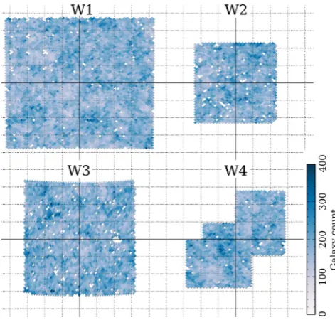
maps for the VIPERS-like colour selection are shown in Fig. 1. We use a survey mask provided by CFHTLS and exclude sources that fall within the haloes of bright stars. For cells that fall on a mask boundary, we measure the fractional coverage using a uniformly spaced grid of 16×16 test points within the cell. We useMANGLE2

Figure 1. Galaxy count maps in the CFHTLS-Wide fields with the VIPERS-like colour selection. We useHEALPIXcells with size 7 arcmin. Gaps in the

survey coverage are left as blank pixels. The grid overlay has spacing of 1◦.

to test if points fall inside the mask (Swanson et al. 2008). This provides us with a weight mapwi=1/fi, wherefiis the fractional

sampling for pixeli. Cells that have less than 50 per cent inclusion in the survey are removed from the map. The areas of the four fields W1, W2, W3 and W4 are 57.7, 18.6, 36.8 and 19.6 deg2_{. After}

putting galaxies in theHEALPIXcells, the number of pixels in the

four maps are 4787, 1592, 3045 and 1651.

Withnigalaxies counted in celli, the overdensity is computed withδi=niwi/n¯ −1. The mean density in a cell, ¯n, is computed from all four fields as ¯n = _iwini/iwi. The variance ofδi, assuming Poisson statistics, isσ2

i =w2i/n¯.

The clustering of foreground stars can be a significant source of systematic error on large angular scales (Ross et al. 2011a). For the CFHTLS, we can estimate the stellar contamination rate indepen-dently in each of the four fields and apply local corrections to the galaxy density. We measure the contamination rate directly in the W1 and W4 fields by counting the number of targets spectroscopi-cally classified as stars in the VIPERS sample. We then extrapolate these rates to the W2 and W3 fields by computing the fraction of sources photometrically classified as stars and then scaling.

The total count in a cell broken down into stars and galaxies is given byNobserved = N + Ngalaxy, and the stellar contamination

fraction is f = N/Nobserved. The values we derive are listed in

Table 2. We apply the correction in the following way: δi,corr = δi/(1−f) andσi,2corr = σ

2

i/(1−f)2(Huterer et al. 2001). The effect on the amplitude of the power spectrum is∼5 per cent.

A fraction of galaxies will also be misclassified as stars and removed from the sample. However, as long as the sample is

Table 2. Star contamination fractions.

Sample W1 W2 W3 W4

SV 0.019 0.056 0.020 0.044 S6 0.013 0.030 0.010 0.017 S7 0.015 0.042 0.015 0.032 S8 0.017 0.055 0.019 0.048 2012 The Authors, MNRAS421,251–261

representative of the full population, the power spectrum measure-ment will not be biased. This may not be the case in reality since misclassified galaxies may preferentially represent a subclass with a different power spectrum amplitude. We do not investigate this correction here.

2.3 Redshift distribution

We use the VIPERS spectroscopic redshift catalogue (internal re-lease, version 1.1) to calibrate the redshift distribution of the pho-tometric samples (see Table 1). In total, we use 13 191 galaxies from VIPERS including 6516 from the W1 field and 6675 from the W4 field. All targets that meet the photometric selection criteria with secure redshifts are used. We select based on the quality flag

zflag. Reliable redshifts havezflagmodulo 10≥2, and we take

zflagin{2..9}(galaxy type),{12..19}(active galactic nucleus) and

{22..29}(serendipitous detections). The flag also has a fractional part indicating agreement with the photometric redshift on a scale from 1 to 5, where 5 indicates good agreement (within 1σ).

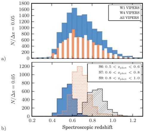
We estimate the redshift distribution from the histogram of spec-troscopic redshifts with a bin size ofz=0.05 (see Fig. 2). We use the histograms directly in the analysis with linear interpolation between bin centres. The redshift distributions of the W1 and W4 samples are remarkably similar despite that these fields are well separated on the sky. We use the distributions from the two fields to test the impact of cosmic variance on our results. As we will con-clude in Section 5.1, small perturbations to the redshift distribution do not strongly impact the results.

The selection function of the VIPERS is not uniform with target apparent flux. There are two sampling rates that we consider: first, the fraction of potential targets that are selected for observation and, second, the fraction of observed targets that give a successful redshift measurement. The first distribution is nearly uniform; the VIMOS spectrograph can place slits on∼40 per cent of the potential targets and this fraction is found to be independent of the magnitude

Figure 2. Redshift distributions of the spectroscopic samples used. (a) The distribution of the full VIPERS sample is shown. Overplotted are the distributions from the W1 and W4 fields individually. (b) The spectro-scopic redshift distributions of the three photometric redshift subsamples are plotted.

of the source. However, we do find that the fraction of targets that have a measured redshift with qualities meeting our criteria drops from 100 per cent at i= 19 to 50 per cent at i= 22.5, the flux limit of the survey. This trend may be corrected for by weighting the contribution of each galaxy in the redshift distribution by the inverse of the sampling rate. However, we find that the correction has a negligible effect on the distribution. Weighting the galaxies shifts the mean redshifts of the samples by less than

z=0.01. We also confirm that lowering the quality threshold of the spectroscopic sample tozflag≥1.5, which adds 11 per cent additional sources, does not significantly alter the distribution. In Section 5.1, we consider the effect of shifting the mean redshift by

z=0.05 to provide an overly conservative check on the effect of uncertainties in the redshift distribution.

3 A N G U L A R P OW E R S P E C T R U M

From galaxy counts in an image, we may infer the projected over-density of galaxies on the sky,δ( ˆn)=₀∞δ3D( ˆn, r)φ(r)r2dr.

Typ-ically, this is an integration through a broad slice in redshift defined by a photometric galaxy selection function or simply by the lim-iting flux of the survey. We expand the density field in spherical harmonics and express the power in modelby the spectrumCl.

We may write the angular power spectrum as a projection of the three-dimensional power spectrum,Pk = δ3D,k2. On large scales, the power spectrum evolves with the linear growth factor,

D1(z). We scale the power spectrum taken at the median redshift of

the sample, ¯z, asPk(z)=[D1(z)/D1(¯z)]2Pk(¯z). This gives

Cl= _π2 φ(r)D1(z)/D1(¯z)jl(kr)r2dr 2

Pk(¯z)d_kk, (1)

wherer is comoving distance. In the small angle approximation, the spherical Bessel function can be approximated as jl(x) =

π 2l+1δ(l+

1

2−x), expressed with a Dirac delta function, and

we find Limber’s equation:

Cl=

gl(k)Pkdk

k . (2)

The projection kernel,gl(k), is given by

gl(k)= _l+1 1/2 r

2_φ(r)D

1(z)/D1(¯z)

2

atr = l+1/2

k . (3)

A correction may be added to account for redshift-space distortions although it is sizable only on large scales atl<50 that we are not sensitive to here (Ross et al. 2011b; Thomas et al. 2011). We may now approach the deprojection problem as a deconvolution of Limber’s equation.

4 P OW E R S P E C T R U M E S T I M AT O R

On large scales, the galaxy density may be described by a Gaussian random field and the distribution is fully characterized by its vari-ance. With this assumption, the likelihood function of the ob-served overdensities on the sky may be written explicitly. We order the mpixels of the density map and form a data vector, x = [δ( ˆn0), δ( ˆn1), . . . , δ( ˆnm−1)], and write the covariance of the

data asCij= xixj. The likelihood function is

L= √ 1

(2π)mdetCexp

−1

2x

T

C−1_x

. (4)

The covariance between the overdensity in pixelsiandjseparated by an angleθij is given by the sum of the signal and the noise

2012 The Authors, MNRAS421,251–261

components:

Cij =

l 2l+1

4π Pl(cosθij)B

2

lCl+Nij, (5)

whereNijis the noise covariance matrix andPlare Legendre poly-nomials. The noise matrix is taken to be diagonal with Poisson elements given byNii = w2i/n¯. The finite resolution of the pix-elized map attenuates the power spectrum by the pixel window function,Bl, which depends on the pixel geometry (G´orski et al. 2005).

We now derive a power spectrum estimator that maximizes the likelihood function, L. The quadratic form was introduced by Tegmark (1997) and explicit derivations have been given in Dodelson (2003, chapter 11), Dahlen & Simons (2008) and Bond et al. (1998). We give an overview here, since many variations exist.

We denote the set of parameters to be estimated by the vectorλ. For our study,λiwill represent a bin of the power spectrum. We begin with an initial estimate,λ(0), and intend to use an optimization algorithm to find a better estimate, ˆλ, that maximizes the likelihood function. With the assumption that lnLhas a quadratic form near the peak, we may apply the Newton–Raphson root-finding method to move towards the peak of the likelihood function (Press et al. 1992), with

ˆ

λ=λ(0)₋ ∂lnL/∂λ

∂2

lnL/∂λ2

λ(0)

. (6)

This expression may be used iteratively to locate the peak. We evaluate the derivative terms in Appendix A, and now simply state the final result for one iteration step:

ˆ

λi= 1 2

j

AijxTEjx−TrEjN, (7)

Ej =C−1_∂∂_λC

jC

−1_.

(8)

The matrixAis a mixing matrix that sets the normalization and may be specified to form linear combinations of the bin estimates. We will use this matrix to shape the window functions. The second term in equation (7) subtracts the noise bias.

We see that the estimator weights the data by their covari-ance:C−1x. This approach has the favourable property that spa-tial modes contribute to the measurement with an inverse-variance weight. The weighting also appropriately ‘tapers’ the map near the mask boundary giving compact window functions in harmonic space.

We have not yet specified the parameter vectorλ. We setλto bins of the three-dimensional power spectrum and evaluate the derivative matrix in equation (8), as

∂Cij ∂λk ≡

∂Cij ∂Pk =

lmax

l=2

2l+1

4π Pl(cosθij)B

2

lgl(k)lnk. (9)

Here, we have replaced the integral in Limber’s equation (equa-tion 2) with a discrete sum over lnk with logarithmic bin widthlnk.

The expectation of the estimate is given by

ˆ

λ =AFλ, (10) where we have introduced the Fisher matrix

Fii= 1 2Tr

C−1∂C

∂λiC

−1∂C

∂λi

. (11)

The variance of the estimate is

Var( ˆλ,λˆ)=AFAT, (12)

and the window functions areW=AF.

The inverse of the Fisher matrix represents the minimum vari-ance that we may hope to achieve on ˆλ. WithA=F−1_{, we see that}

we have an estimator that is optimal in the sense that it is unbiased and has minimum variance (Tegmark 1997). This approach may not be practical, however, because the Fisher matrix is often singular or numerically ill conditioned. Intuitively, this reflects the funda-mental limit that we cannot probe the power spectrum at scales smaller than∼ (θ)−1_{, whereθ is the angular size of the}

survey.

Instead, we chooseAwith the aim of diagonalizing the covariance matrix. By factoring the Fisher matrix asF= MMT, we can set A=M−1_{. The covariance matrix is now Var( ˆλ,λˆ)=}

M−1FM−1T.

In practice, we computeMas the square root of the Fisher ma-trix using an SVD method. We also rescaleM to normalize the window functions such that _jWij = 1. This approach was shown by Tegmark (1997) to result in sharper window func-tions than the common choice for A, a diagonal matrix with

Aii=[jFij]−1_.

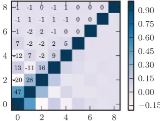
We find that the matrixMis ill conditioned when the window functions are broad, especially for the SV sample which has a wide redshift distribution. To find a stable inversion, we use a pseudo-inverse technique by keeping only the largest singular values. The consequence of using a pseudo-inverse is that the covariance matrix will not be perfectly diagonalized. The covariance matrix for the VIPERS estimate after carrying out this operation is shown in Fig. 3. The choice of how many modes to keep in the pseudo-inverse affects the shape of the window functions and the scales that are probed. We find that the smaller singular values probe large scales, in the same fashion as in the SVD analyses by Eisenstein & Zaldarriaga (2001) and Maller et al. (2005). We set the scale ensuring that the resulting window functions are positive and reach the largest scales available to the survey.

The estimate and covariance model depend on the chosen fidu-cial cosmology through the form of the likelihood function and the projection kernel. Both the shape and normalization of the power spectrum can be important. Although the normalization cancels in the estimator (neglecting the noise term), it is important for the Fisher matrix and covariance. For these reasons, maximum likeli-hood estimators are often applied iteratively to arrive at consistent results. We explore these dependencies with simulations in the next section.

Figure 3. The correlation matrix forPkestimated from the VIPERS-like

sample. Elements of the matrix are labelled with the per cent correlation. Although the window functions overlap significantly, the bins are nearly statistically independent by construction.

2012 The Authors, MNRAS421,251–261

5 S I M U L AT I O N S

5.1 Gaussian realizations

As a test of the method, we estimate the power spectrum for Gaussian realizations of the projected density field. The simula-tions are constructed using aCAMBpower spectrum with the Halofit

model (Lewis, Challinor & Lasenby 2000; Smith et al. 2003) and projected through the VIPERS redshift distribution. With theseCl, we use HEALPIXSynfast to generate simulated density maps. We

produced 1000 independent maps with a resolution of 7 arcmin (nside=512). We add noise fluctuations by drawing from a

Gaus-sian distribution assuming a variance given by Poisson statistics with ¯n= 50 galaxies per cell. This is a higher level of noise than we find in the CFHTLS catalogue. For the geometry of the mock survey, we use the actual survey mask of the W2 field. It includes 1592 pixels covering 21 deg2_.

We compute the Fisher matrix in logarithmic bins fromk=0.01 to 100 withlogk =0.05. The results are plotted in Fig. 4. The

data points are rebinned tologk=0.1 and plotted fromk=0.06

to 0.7hMpc−1_{. The corresponding window functions are shown in}

the bottom panel. The data are plotted at the peaks of the window functions. On large and small scales, the window functions begin to overlap and converge as the limits set by the survey geometry are reached. On small scales, we see a secondary peak in the window function atk∼2hMpc−1_{which arises from the pixel scale of the}

map (see Fig. 5).

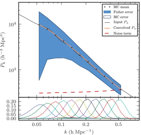
We convolve the theory power spectrum with the window func-tions and find that the mean of the Monte Carlo runs agrees well within a few per cent. We expect that the precision is limited by the finite binning of the Fisher matrix and truncation of the window functions, but these effects are well below the statistical uncertain-ties. The errors computed analytically from the Fisher matrix agree with the distribution of Monte Carlo runs to within a few per cent.

Figure 4. The top frame shows the recovered power spectrum from the mean of 1000 independent Gaussian simulations. The theory is convolved with the window functions (plotted at bottom) and we find that it matches the measurement to within a few per cent. The error bars computed analytically from the Fisher matrix (shaded area) agree with the distribution of Monte Carlo runs (outline). The noise term in equation (7) is shown as a dashed curve.

Figure 5. In the top panel, we plot the projection kernels,gl(k). We compare

the kernels derived from the W1 redshift distribution only (solid curves) and those from W4 only (dashed curves). Lower panel: the window functions found for the 21 deg2_{simulation field are plotted. To check robustness, we}

again compare the results derived from the W1 and W4 fields separately. The second peak in the window functions atk>1hMpc−1_{arises from the}

pixel scale of the map; beyondk=2hMpc−1_{, the window functions rapidly}

drop to 0.

These errors are for a single field, and so we can expect to achieve a factor of 2 better with the combination of four fields.

5.2 Dependence on redshift distribution

We checked the robustness of the measurement to uncertainties in the redshift distribution by repeating the analysis with different assumed distributions. The simulations were generated with the measured redshift distribution from the complete VIPERS sample, and we first reanalysed them with distributions derived from two subsamples, the redshift distribution of W1 and W4. The numbers of spectra taken in the two fields are similar and the spectroscopy covers similar areas, but the fields are widely separated on the sky and so any differences could be attributed to cosmic variance. We compute the Fisher matrix using the two distributions and find that the projection kernels and window functions agree (Fig. 5). The bias introduced by a mismatched redshift distribution is at the per cent level, below the statistical errors.

Additionally, the measured redshift distribution could be inac-curate due to sampling biases in the VIPERS. In Section 2.3, we concluded that the uncertainty in the mean redshift of the distri-bution, ¯z, is known to be better than z = 0.01. As an overly conservative check, we examine the consequences of shifting the redshift distribution byz= ±0.05. This was done by modulat-ing the measured distribution of the full VIPERS sample by the linear functionf(z)=1±1.5(z−z¯). The modified distributions have ¯z1 = 0.656 and ¯z2 = 0.752, while the original sample has

¯

z=0.703 (see the lower panel of Fig. 6). We find that reducing ¯z by 7 per cent lowered the derived power spectrum by 10 per cent. Increasing ¯z by 7 per cent increased the power spectrum by 6 per cent. This large shift in ¯zwould thus lead to a systematic error in the estimated bias factor at the level of 3–5 per cent.

2012 The Authors, MNRAS421,251–261

Figure 6. The influence of the assumed redshift distribution on the deprojec-tion. Top panels: the simulations are analysed with the W1 and W4 redshift distributions. Bottom panels: for an overly conservative test, we modify the VIPERS redshift distribution to adjust the mean redshift byz= ±0.05 (labelled Test 1 and Test 2), leading to systematic shifts in the amplitude of the estimated power spectrum of+6 and−10 per cent. The redshift distri-butions are plotted in the right-hand panels and the derived power spectra are on the left. In the top and bottom, the filled grey distribution represents the redshift distribution of the full VIPERS sample.

5.3 Dependence on fiducial cosmology

The dependence on the fiducial cosmology enters the analysis in two ways. First, we rely on the cosmology to model the likelihood function. In the maximum likelihood estimator, the data covariance matrix plays the role of a weight. Modifying the fiducial power spectrum changes the weighting function and could bias the esti-mator. We can expect that assuming the wrong matter density, for example, could bias the estimator and make the variance properties suboptimal.

The second dependence on the fiducial cosmology is through the projection kernel. In the previous section, we discussed how shifting the redshift distribution affects the amplitude of the power spectrum estimate. We can expect that varying the cosmology and the redshift–distance relation will have a similar effect.

Our Gaussian simulations were constructed using the reference

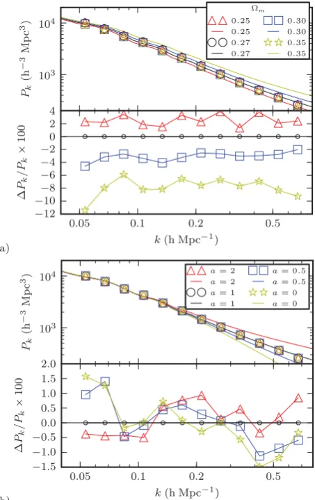
CDM power spectrum with the Halofit model. To test the depen-dence on the cosmology, we first reanalyse the maps using fiducial power spectra with different assumed values of the matter den-sity, takingm=0.25, 0.30 and 0.35. All other parameters were

held fixed at the reference values. We find that despite assum-ing the wrong matter density, we recover the correct shape of the power spectrum from the mean of 1000 simulation runs to within 2 per cent (see Fig. 7, panel a). However, it is clear that the amplitude is strongly biased. This is due to the dependence of the projection kernels onm. This geometric dependence on the background

cos-mology dominates over any bias in the estimator due to suboptimal weighting. These findings support an iterative approach.

Next, we check the influence of variations in the amplitude of the power spectrum at small scales. The shape of the power spectrum on small scales has developed with the aid ofN-body simulations but it remains a source of systematic uncertainty. We vary the small-scale amplitude using an interpolation parameteranl:

˜

Pk=Pk,lin+

Pk,nl−Pk,lin

anl. (13)

We test a range of amplitudes withanl={0, 0.5, 1, 2}(anl=1 gives the Halofit model). We find that the estimator is remarkably robust

Figure 7. The sensitivity of the estimator to the assumed fiducial model. (a) We varymkeeping other parameters fixed. The top frame shows the fiducial power spectra (solid lines) and the points mark the derived power spectrum measurements. The bottom frame shows the per cent differences from the reference model for each trial. The correct shape is recovered, but there is a shift in the amplitude of the estimate due to the geometric dependence of the projection kernel on the cosmology. (b) We modulate the small-scale amplitude of the fiducial power spectrum with an interpolation parameteranl;anl=0 and 1 correspond to the linear and Halofit models,

respectively. We find that the derived power spectrum is not sensitive to the small-scale amplitude.

(see Fig. 7, panel b). The discrepancy introduced by the variation in the small-scale amplitude is less than 2 per cent on large scales and it is dominated by numerical uncertainties up tok∼0.2hMpc−1_.

This supports the conclusion that using suboptimal weights does not significantly bias the result.

6 R E S U LT S

We now carry out the estimation of the power spectrum on the CFHTLS data for the VIPERS-like sample and three photometric redshift subsamples (see Fig. 8). For the analysis, a fiducialCAMB

power spectrum with the Halofit model is assumed. The Fisher matrix is computed with 60 bins logarithmically spaced fromk=

0.01 to 10 withlogk=0.05. We use a widek-range to map out the window functions but all these data are not useful for analysis. We restrict the study to 13 points fromk=0.03 to 0.6hMpc−1_{. We can}

2012 The Authors, MNRAS421,251–261

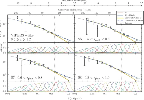
Figure 8. The deprojected three-dimensional power spectrum in logarithmic bins for the VIPERS-like sample and three photometric redshift selected samples:

zphot=0.5–0.6, 0.6–0.8 and 0.8–1.0. The window function of each band is shown in the panel below each plot. The theoretical power spectrum (both linear

and Halofit models) is convolved with the window function and overplotted with the best-fitting linear bias listed in Table 3. We use the first nine data points, up tok0.2hMpc−1_{indicated by the vertical dotted line, to estimate the linear bias. The corresponding comoving distance and angular scale (atz=0.7) are}

included as a guide.

go to smaller scales, although the Gaussian error estimate will not be appropriate. We use a bin size oflogk=0.1 which is appropriate choice considering the width of the survey window functions. The plotted error bars are derived from the diagonal elements of the covariance matrix found computed from equation (12).

For each field, we compute the normalized quantity from equa-tion (7),y_jk = 1

2{x T

Ejx−Tr (EjN)}, wherekindexes the fields 1–4, along with the Fisher matrix (equation 11). These results are then summed together, and the final combined estimate is computed by ˆλi= 12

4

k=1

jAijyjk, whereA=(

4

k=1Fk)−1/2normalized

such that_i(AF)ij = 1. This combination properly weights the data. The covariance of the estimate for the VIPERS-like sample is shown in Fig. 3. At lowk, neighbouring bins are nearly 50 per cent correlated, but the matrix becomes more diagonal at largerk. The limitation in diagonalizing the covariance matrix comes in the inver-sion ofM=F1/2_{. This is computed with a pseudo-inverse method.}

The inversion becomes easier for the narrower photometric redshift slices where a nearly perfect inversion is possible. The window functions are sharper for these redshift slices as well.

We do not run the maximum likelihood algorithm in an iterative fashion. The data do not support strong constraints onCDM pa-rameters alone and we find that beginning with a fiducialCDM power spectrum, we have a very good fit to the data. This indicates

that our starting point is already near to the peak of the (very broad) likelihood function. However, we do effectively carry out one itera-tion of the estimator to find the galaxy bias and set the amplitude of the fiducial power spectrum. This is necessary because the estimator and covariance do not simply scale linearly with amplitude in the presence of noise. A second run allows us to set the amplitude of the fiducial power spectrum ensuring that the error estimate is correct. We compute a one-parameter fit to estimate the galaxy bias on linear scales. We restrict this fit to the first nine points at k < 0.2hMpc−1_{. Given the Pk measurements in vector d}

and the convolved CDM model in vector m, we find the amplitude, a, that maximizes the likelihood function, lnL =

−1/2 (d−am)TC−kk1(d−am). The solution is given by

a= d T

C−kk1m

mT_C−1

kkm

, (14)

with variance σ2

a =

mT

C−kk1m −1

. The resulting values of the galaxy bias are listed in Table 3, where we have assumed a value of

σ8=0.8. The bias increases with redshift as expected for a

flux-limited survey. In fact, the amplitude of the power spectrum is not seen to change with increasing redshift, indicating that the evolution of the growth factor and the galaxy bias factors approximately

2012 The Authors, MNRAS421,251–261

Table 3. Best-fitting galaxy bias.

Sample bg χ2

VP: VIPERS-like 1.38±0.05 7.2 S6: 0.5<zphot<0.6 1.36±0.05 7.1

S7: 0.6<zphot<0.8 1.52±0.05 5.7

S8: 0.8<zphot<1.0 1.68±0.05 2.0

cancel. We find an approximately constant error on the bias factor in each redshift range; this is simply due to the fact that the amplitude of the fiducial power spectrum (from which the errors are derived) is approximately constant.

Also in Table 3, we list theχ2_{values at the best fit. The number of}

degrees of freedom is approximately 8. Theχ2_{values are lower than}

expected, specifically for S8 for which we findχ2_{=2. Formally,}

the probability of findingχ2_{≤2 with eight degrees of freedom is}

0.019. This could indicate that the covariances, and consequently the error bars, are overestimated for this sample.

7 PA R A M E T E R E S T I M AT I O N

Before we may carry out a joint analysis, we must estimate the covariance between the overlapping photometric samples. We will estimate the covariance of the estimators with a Fisher matrix ap-proach in the full-sky limit and then rescale to find the errors for our survey geometry.

We compute the covariance between two samples labelledAand

B. To simplify the expression, we write the product of the kernel with the beam and integration step as ˜gl(k) = gl(k)B2

llnk and

the sum of the signal and noise covariance as ˜Cl=ClBl2+n¯ . It

is more convenient to use the harmonic space representation, and we switch the data vector fromxitoalm. The covariance matrix is diagonal:Clm;lm=δllδmmC˜l.

A component of the Fisher matrix for a single sampleAfor two power spectrum bins,kandk, is

FA,kk=

l 2l+1

2 g˜ A l(k) ˜glA(k)

˜

ClA −2

. (15)

We can write the quadratic estimator for the power spectrum as

ˆ

PA k =

1 2

k

F−1

A,kk

lm

a2

lmg˜lA(k)

˜

ClA −2

. (16)

We find the covariance between the two sample estimates to be

Cov( ˆP_kA,Pˆ_kB)= 1

fsky

h,i,j

F−1

A,kiFB,ij−1

×

l 2l+1

2 g˜ A l(j) ˜gBl(k)

˜

ClAB ˜

ClAC˜lB

2

. (17)

We scale by the fractional sky coverage of the survey,fsky, which

ap-proximately accounts for the number of modes that may be probed. The small survey size also broadens the window functions, which we account for in the covariance withCkk=WACkkWBT.

The variances for one sample computed with equation (17) in the full-sky limit match well with the full computation of the Fisher matrix (equation 12) (see Fig. 9). Although, we find that the full-sky computation underestimates the variance by a factor of∼2. This is not surprising since we have neglected the precise survey geometry. As a correction, we rescale the estimate to match the variance in the S7 slice. In Fig. 9, we also show the analytic estimates of the

Figure 9. The covariance between the photometric redshift samples is plotted. The circle markers show the full computation of the variance of the S7 slice that accounts for the survey geometry. The solid curves show the analytic Fisher approximation in the full-sky limit (equation 17). Inset is the full correlation matrix for the three samples.

covariances between the three redshift slices that we may now use to perform a joint likelihood analysis.

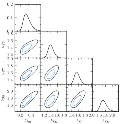
Using the sample covariances, we jointly estimate the linear galaxy bias factors of the three photometric redshift slices, S6, S7 and S8, labelled asbS6,bS7andbS8along withm. All other CDM parameters are held fixed and we setσ8=0.8. We

com-pute the likelihood of a model with the full covariance matrix. The fit is limited to the first nine data points of each sample, giving a maximumkofkmax=0.2hMpc−1. We exhaustively evaluate the

likelihood over the four-dimensional parameter grid. Views of the likelihood surface, marginalized over pairs of parameters, are shown in Fig. 10. The marginalized constraints are listed in Table 4 with 68 per cent confidence intervals.

Figure 10. The joint likelihood surfaces ofmand the bias parameters for the three photo-zsamples (bS6,bS7,bS8). The inner and outer contours

indi-cate the 68 and 95 per cent confidence level. The marginalized likelihoods of each parameter are listed in Table 4. The fit is limited to the first nine data points, givingkmax=0.2hMpc−1.

2012 The Authors, MNRAS421,251–261

Table 4. Marginalized parameter estimates.

m 0.30±0.06

bS6 1.39±0.08

bS7 1.55±0.08

bS8 1.72±0.10

The joint analysis prefers a slightly higher value ofm, 0.30±

0.06, versus the fiducial model with 0.272. Due to the correlations between parameters, this results in higher values of the galaxy bias factors than were found with the fiducial model fixed (Table 3).

8 C O N C L U S I O N S

The CFHTLS-Wide fields probe a significant cosmological volume at redshifts not reached by other galaxy surveys to date. We use the projected density field from photometric redshift samples to constrain the real-space power spectrum and derive constraints on the matter density and linear galaxy bias factors. These results are made possible by precise knowledge of the redshift distributions provided by preliminary results from the VIPERS.

The primary advantage of computing the power spectrum directly from the angular distribution, instead of using conventional spher-ical harmonicsCl, is that we may construct window functions in Fourier space. By optimizing this, we achieve sharper constraints on the power spectrum than when we are limited tobands. This approach comes with the cost that we must adopt a fiducial power spectrum. We showed that using the wrong fiducial power spectrum, although leading to suboptimal weights, does not significantly bias the estimate. This is true even on small scales, and we can ef-fectively use this method to deconvolve small and large scales in Limber’s equation. Residual systematic error on the derived power spectrum is at the 1 per cent level, well below the sensitivity of the measurement.

The deprojection does strongly depend on the assumed redshift distribution of the galaxy sample as well as the cosmology used to compute the redshift–distance relation. The cosmology dependence of the measurement makes the interpretation difficult, but to a first approximation, only the amplitude is affected; the shape of the power spectrum is recovered correctly. Thus, a converging iterative procedure can be implemented by updating the fiducial model and repeating the analysis.

There is a degeneracy between a shift in the assumed redshift distribution and the cosmological model. This is unavoidable when studying a field in projection. However, the constraints on the red-shift distribution can always be improved with further observation. In our analysis, from the sampling biases present in the VIPERS spectroscopy, we estimate the uncertainty in the mean redshift to be at the 1 per cent level. Thus, we do not expect a strong systematic error in the derived galaxy bias parameters. We do note that the observed trend of lowχ2_{values for the best-fitting models in the}

higher redshift samples can arise if the covariance is overestimated. This could be a weak hint that the true mean redshift is lower than what we assume or that a modification is needed in the fiducial cosmology.

Recently, the galaxy bias was measured from the CFHTLS-Wide fields in the context of the halo model by Coupon et al. (2011). Our final two photometric redshift bins, S7 and S8, correspond to samples constructed by Coupon et al., so we are able to compare the resulting bias values. Coupon et al. constructed volume-limited samples using luminosity cuts, resulting in a selection of brighter

galaxies; thus, we may expect their bias values to be larger. The halo model constraints of Coupon et al. (2011) give for S7bg=

1.44±0.01 and for S8bg=1.79±0.03. These values have been

scaled by 1.03 to transform from a cosmology withm=0.25 to

0.272 which is assumed here. Our value ofbgfor the S7 sample

is higher, while for the S8 sample it is lower, although both are in agreement with Coupon et al. within the 2σ confidence limit. The measurements are based on different physical scales (Coupon et al. restrict the correlation function to angular scales<1◦.5) and different model assumptions have been used. Thus, it is reasonable to consider the measurements as independent estimates.

Our results provide a preliminary look at the large-scale structure field probed by the VIPERS colour selection and demonstrate the strengths of the VIPERS sample for clustering studies atz>0.5. We anticipate promising results with the full VIPERS spectroscopic sample.

AC K N OW L E D G M E N T S

We are grateful to the VIPERS team for supporting this project. In particular, we thank Lauro Moscardini for suggestions that im-proved the work. We thank Jian-Hua He for carefully reading the manuscript. We acknowledge the support of INAF through a PRIN 2008 grant. The computational methods used were inspired by Istv´an Szapudi’s mlhood code. Our results are derived with

COSMOPY(www.ifa.hawaii.edu/cosmopy) andHEALPIXwith Healpy (healpix.jpl.nasa.gov, code.google.com/p/healpy). This work is based on data obtained with the European Southern Observatory Very Large Telescope, Paranal, Chile, programme 182.A-0886. This work is also based on observations obtained with MegaPrime/ MegaCam, a joint project of CFHT and CEA/DAPNIA, at the Canada–France–Hawaii Telescope (CFHT) which is operated by the National Research Council (NRC) of Canada, the Institut National des Sciences de l’Univers of the Centre National de la Recherche Scientifique (CNRS) of France and the University of Hawaii. This work is based in part on data products produced at TERAPIX and the Canadian Astronomy Data Centre as part of the Canada–France– Hawaii Telescope Legacy Survey, a collaborative project of NRC and CNRS.

R E F E R E N C E S

Baugh C. M., Efstathiou G., 1993, MNRAS, 265, 145 Baugh C. M., Efstathiou G., 1994, MNRAS, 267, 323

Blake C., Collister A., Bridle S., Lahav O., 2007, MNRAS, 374, 1527 Bond J. R., Jaffe A. H., Knox L., 1998, Phys. Rev. D, 57, 2117 Coupon J. et al., 2009, A&A, 500, 981

Coupon J. et al., 2011, preprint (arXiv e-prints)

Dahlen F. A., Simons F. J., 2008, Geophys. J. Int., 174, 774

Dodelson S., ed., 2003, Modern Cosmology. Academic Press, Amsterdam Dodelson S., Gazta˜naga E., 2000, MNRAS, 312, 774

Dodelson S. et al., 2002, ApJ, 572, 140

Efstathiou G., Moody S. J., 2001, MNRAS, 325, 1603 Efstathiou G. et al., 2002, MNRAS, 330, L29 Eisenstein D. J., Zaldarriaga M., 2001, ApJ, 546, 2 Fu L. et al., 2008, A&A, 479, 9

Gazta˜naga E., Baugh C. M., 1998, MNRAS, 294, 229

Goranova Y. et al., 2009, The CFHTLS T0006 Release (http://terapix.iap.fr/ cplt/T0006-doc.pdf)

G´orski K. M., Hivon E., Banday A. J., Wandelt B. D., Hansen F. K., Reinecke M., Bartelmann M., 2005, ApJ, 622, 759

Huterer D., Knox L., Nichol R. C., 2001, ApJ, 555, 547 Kilbinger M. et al., 2009, A&A, 497, 677

Larson D. et al., 2011, ApJS, 192, 16

2012 The Authors, MNRAS421,251–261

Lewis A., Challinor A., Lasenby A., 2000, ApJ, 538, 473

Maddox S. J., Efstathiou G., Sutherland W. J., Loveday J., 1990, MNRAS, 242, 43p

Maller A. H., McIntosh D. H., Katz N., Weinberg M. D., 2005, ApJ, 619, 147

Padmanabhan N. et al., 2007, MNRAS, 378, 852

Press W. H., Teukolsky S. A., Vetterling W. T., Flannery B. P., eds, 1992, Numerical Recipes in FORTRAN. The Art of Scientific Computing. Cambridge Univ. Press, Cambridge

Ross A. J. et al., 2011a, MNRAS, 417, 1350

Ross A. J., Percival W. J., Crocce M., Cabr´e A., Gazta˜naga E., 2011b, MNRAS, 415, 2193

Shan H. et al., 2011, preprint (arXiv e-prints) Smith R. E. et al., 2003, MNRAS, 341, 1311

Swanson M. E. C., Tegmark M., Hamilton A. J. S., Hill J. C., 2008, MNRAS, 387, 1391

Szalay A. S. et al., 2003, ApJ, 591, 1 Tegmark M., 1997, Phys. Rev. D, 55, 5895 Tegmark M. et al., 2002, ApJ, 571, 191

Tegmark M. et al., 2004, Phys. Rev. D, 69, 103501

Tereno I., Schimd C., Uzan J.-P., Kilbinger M., Vincent F. H., Fu L., 2009, A&A, 500, 657

Thomas S. A., Abdalla F. B., Lahav O., 2011, MNRAS, 412, 1669

A P P E N D I X A : Q UA D R AT I C E S T I M AT O R

In Section 4, we reasoned that we would apply the Newton–Raphson root-finding algorithm (equation 6) to locate the peak of the like-lihood function (equation 4). We now continue and evaluate the derivatives of the likelihood function,∂lnL

∂λi and

∂2_lnL

∂λi∂λj. We assume

that the covariance of the data depends linearly on the parameters

Cij=kPk,ijλk+Nij. The first derivative term is ∂lnL

∂λi =

∂ln detC

∂λi +x

T∂C− 1

∂λi x (A1)

=Tr

C−1_∂∂_λC i

−xTC−1_∂∂_λC iC

−1

x. (A2)

Two identities have been used: ln (detC)=Tr (lnC) and ∂C_∂λ−1 =

−C−1∂_∂C_λC−1. The second derivative, or curvature, is ∂2

lnL ∂λi∂λj = −Tr

C−1_∂∂_λC

iC

−1∂C

∂λj

+2xT

C−1_∂∂_λC iC

−1∂C

∂λjC

−1

x.

(A3)

We neglect the second derivative terms. To simplify, we replace the curvature by its average over an ensemble of realizations of the data. This is known as the Fisher matrix:

Fij ≡ 1 2

∂2_lnL

∂λi∂λj

= 1

2Tr

C−1_∂∂_λC iC

−1∂C

∂λj

. (A4)

Inserting these expressions into equation (6), we find that one iteration step in the Newton–Raphson algorithm is given by

ˆ

λi=λ(0)i −

j

∂2

lnL ∂λi∂λj

−1

∂lnL

∂λj (A5)

=λ(0)

i +

j

∂2_lnL

∂λi∂λj −1

×

xTC−1_∂∂_λC iC

−1

xT−Tr

C−1_∂∂_λC

i

(A6)

=λ(0)

i + 1 2

j

F−1

ij

xT

C−1_∂∂_λC iC

−1

x−Tr

C−1_∂∂_λC i

.

(A7)

The terms on the right are computed with the parameter setλ(0)_{. We}

may simplify further by rewriting the trace term with

C−1_∂∂_λC i =C

−1∂C

∂λiC

−1

C (A8)

=

k

C−1_∂∂_λC iC

−1

_∂

C

∂λkλk+N

(A9)

=2 k

Fikλ(0)k +C−1_∂∂_λC iC

−1

N, (A10)

where we use the linear dependence ofCon the parameters. Sub-stituting into (A7), the product of the Fisher matrix with its inverse leads to a cancellation of theλ(0)_{terms. We are left with the final}

estimator in quadratic form:

ˆ

λi= 1 2

j

F−1

ij

xT

C−1∂C

∂λiC

−1_x−Tr

C−1∂C

∂λiC

−1

N

.

(A11)

This paper has been typeset from a TEX/LA_{TEX file prepared by the author.}

2012 The Authors, MNRAS421,251–261