on C
−60anions
Elie A. Moujaes and Janette L. Dunn‡
School of Physics and Astronomy, University of Nottingham, Nottingham, NG7 2RD, UK.
Abstract. Singly-charged buckminster fullerene anions, C−
60, are subject to a strong
intramolecularT⊗hJahn-Teller (JT) effect. When such ions interact with other C−
60
ions in a solid through a co-operative JT effect, they will be subject to an additional interaction. There are a number of different mechanisms that can cause this interaction. However, in the molecular field approximation, all can be modelled phenomenologically in terms of a symmetry-lowering interaction written in terms of a linear combination of electronic operators for thehmodes involved in the intramolecular JT effect. We will consider the combined effect of this distortion and the intramolecular JT effect. We will analyse the lowest adiabatic potential energy surface, and calculate the energies of the resultant vibronic states. The results are shown to have a complicated dependence on the particular combination of h modes chosen, and the energies of the resultant vibronic states can not easily be deduced from the form of the potential alone.
PACS numbers: 71.70.Ej,61.48.-c
Submitted to: J. Phys.: Condens. Matter
1. Introduction
Solids formed by combining C60 fullerene molecules and alkali metals to form solids
of the type AnC60 (n = 1 to 6) have a number of unusual and intriguing physical
properties. A3C60 solids show unexpected conducting and superconducting properties
[1, 2, 3], with K3C60 being superconducting at temperatures below 18K, Rb3C60 below
28K and Cs3C60 below 47K [4]. In contrast, A4C60 compounds are insulators. AC60
compounds form a polymeric structure in ambient conditions, with RbC60 and CsC60
undergoing a metal-insulator phase transition at Tc ∼50 K and Tc ∼40 K respectively
[5, 6, 7].
The structure of AnC60solids can also vary. Many of these materials are face centred
cubic (fcc) structures, but some are body centred tetragonal (bct) and body centred cubic (bcc) structures. The low temperature structure of AC60 is orthorhombic with an
unusually short separation of 9.1˚A- 9.4˚A between the centres of C60 molecules along one
of the crystallographic directions [8]. In addition, amorphous-carbon structures based on linearly polymerized C60 molecules have been found under a pressure above 5 GPa
[9, 10]. In a cluster of A3C60 molecules at room temperature, when the fcc solid form of
C60 is maintained, the molecules rotate randomly about their lattice positions between
different orientations. In fact the rotational levels are much closer to each other than the vibrational levels, meaning that the molecules populate the rotational levels much more easily. However, at temperatures lower than 261K, two of the rotational degrees of freedom freeze out, resulting in a lowering of symmetry and merohedral order [11, 12]. Similar conclusions have also been found in compounds containing C2−
60 ions [13].
Influence of the vibrational motion of the C60 molecule on the electronic motion is
known to be important in these fullerene systems. Isolated fullerene ions Cn−
60 (n = 1
to 5) are subject to an intramolecular Jahn-Teller (JT) effect of the form T ⊗h, where a triply degenerate electronic state T is coupled to a five dimensional vibrational mode
h [14]. The JT effect causes an instantaneous distortion of the icosahedral C60 cage to
a lower symmetry. However, there are a number of different distorted configurations all having the same energy. Quantum-mechanical tunnelling between the equivalent configurations restores the icosahedral symmetry in the dynamical JT effect. However, to understand the properties of fullerene solids, it is necessary to go beyond studies of isolated fullerene centres and to consider interactions between fullerene centres and/or interactions with a surface. There are various possible mechanisms for producing interactions between C60ions in C60 solids. One factor which is believed to play a major
role in determining the contrasting behavior of A3C60, A4C60 and AC60 compounds is
the co-operative JT (CJT) interaction between the different ions [15]. As a result of the CJT effect, different possible JT distortions are no longer equivalent and so the dynamical JT effect does not prevail in the lattice. JT distortions of individual centres can be locked in place and in general the lattice configuration will consist of a periodic arrangement of statically distorted ions [16].
interactions between JT centres, some of which involve phonons and some of which do not. In all cases, the interaction Hamiltonian Hij between centres i and j can be
represented phenomenologically (independent of the mechanism involved) using terms quadratic in the collective displacementsQiλandQjλof the vibrationally-coupled modes λ at sites i and j, or equivalently a form quadratic in the electronic operators σiλ and σjλ used to describe the intramolecular JT interaction at sites i and j [15, 16]. One
way to proceed is to then use the molecular field approximation. After making some appropriate transformations, this results in a mean-field Hamiltonian Hmfi for site i
which is equivalent to the intramolecular JT Hamiltonian for site i plus an additional contribution Hs=−Pλwλσλ, where the wλ are constants whose values depend on the
form of the interaction [16, 17]. The result for centreiis the same Hamiltonian as would be used for an intramolecular JT effect plus an additional symmetry-lowering distortion. The latter is sometimes referred to as a ‘strain’, although the origin of this term will not be that of an external stress on the system [15].
In this paper, we will be concerned with JT effects experienced by fullerene anions C−
60. From group theory, coupling of isolated ions to two ag and eight hg vibrational
modes is allowed. However, the coupling to theag modes does not have any significance,
and for most purposes the coupling to the eight hg modes can be replaced by coupling
to a single effective mode [18]. Therefore, the relevant intramolecular JT effect for C−60 is aT1u⊗hg system [14]. The nuclear coordinatesQλ thus correspond to the vibrational
mode hg. By convention, the components λ are denoted by {θ, ǫ,4,5,6} [19]. We will
consider a linear intramolecular JT effect subject to an additional symmetry-lowering distortion that can be written in terms of the electronic operators σλ relevant to the h mode in this system. The distortion can act along the direction of any one of the components λ, or along a linear combination of these directions. We will analyse the shape of the lowest adiabatic potential energy surface (LAPES) in different situations in order to understand the effect of the direction of the distortion, and investigate how the energies of the resultant vibronic states vary with the magnitude and direction of the distortion.
2. The Hamiltonian
The total Hamiltonian of a linear T ⊗h JT system subject to an additional symmetry-lowering interaction Hs is H = Hvib+Hint+Hs, where Hvib and Hint are vibrational
and electron-phonon interaction terms respectively, given by
Hvib =
1 2
X
ν
P2
λ
µ +µω
2
HQ
2
λ
σo
Hint=kH
X
λ
Qλσλ. (1)
λ is summed over the five vibrational degrees of freedom {θ, ǫ,4,5,6}. Qν and Pλ are
the collective coordinates and their conjugate momenta respectively. kH is the linear
of vibration. σo is the identity matrix in three dimensions. Explicitly, we can write
[14, 20, 21]
Hint= kH
2
Qθ−
√
3Qε −
√
3Q6 − √
3Q5 −√3Q6 Qθ+
√
3Qε −
√
3Q4
−√3Q5 −
√
3Q4 −2Qθ
(2)
from which the definitions of the electronic interaction matrices σλ can be deduced.
When defined in this manner, kH is equivalent to the coupling constant k of Ref. [14],
and is related to the constant VH used in Ref. [21] by the relation kH =−2VH/
√
10.
2.1. Separation of coordinates
When linear JT effects only are included in the T ⊗h problem, the LAPES contains a four-dimensional trough of equivalent-energy points. The motion of a system subject to this JT effect will consist of vibrations across and rotations of a distortion around the trough, often called pseudorotations. These should not be confused with the real rotations of the molecule. The trough has SO(3) symmetry, which is accidentally higher than the Ih symmetry expected for the T ⊗ h problem. Due to this symmetry, it is
useful to write the Qλ in the polar form [14, 20]
Qθ =ρ
1 2(3 cos
2θ−1) cosα+ √
3 2 sin
2θsinαcos 2γ !
Qǫ =ρ
√
3 2 sin
2θcos 2φcosα
−cosθsin 2φsinαsin 2γ
+1
2(1 + cos
2θ) cos 2φsinαcos 2γ
Q4 =ρ
√
3
2 sin 2θsinφcosα− 1
2sin 2θsinφsinαcos 2γ−sinθcosφsinαsin 2γ
!
Q5 =ρ
√
3
2 sin 2θcosφcosα− 1
2sin 2θcosφsinαcos 2γ+ sinθsinφsinαsin 2γ
!
Q6 =ρ
√
3 2 sin
2θsin 2φcosα+ cosθcos 2φsinαsin 2γ
+1
2(1 + cos
2θ) sin 2φsinαcos 2γ
, (3)
where ρ is the radial distance, (θ, φ, γ) are Euler angles, and α is an extra angle to complete the five dimensional Q-space. [14, 20] For all points to be included once only, we can choose 0≤ ρ <∞, 0 ≤φ ≤2π, 0≤θ≤π, 0≤γ ≤2π and 0≤α < π/3.
Hamiltonian Heint=RHintR
−1
takes the diagonal form
e Hint=
kHρ
2
cosα−√3 sinα 0 0
0 cosα+√3 sinα 0
0 0 −2 cosα
. (4)
From this, it can be seen that the lowest eigenvalue is lowest of all when α = 0. [14] Also, the eigenvalue is independent of the angles θ, φ and γ, which is consistent with the interpretation of the LAPES being a trough.
If we explicitly write Pλ = −i~ ∂/∂Qλ, the vibrational Hamiltonian in the
five-dimensional polar coordinates becomes
Hvib =
"
− ~
2
2µρ2
∂ ∂ρ
ρ2 ∂ ∂ρ + 1 2µω 2 Hρ
2+ Lˆ2
6µρ2 #
σo (5)
where ˆL2 is the usual angular momentum operator
ˆ
L2 =−~2
1 sinθ ∂ ∂θ
sinθ∂ θ
+ 1
sin2θ
∂2
∂φ2
. (6)
The transformed Hamiltonian for the additional distortion Hs is a complicated result
involving θ, φ and γ. However, we can make the approximation that mixing between the different APESs due to the additional distortion can be neglected. This gives us the contributions
Wθ =
1
4wθ(1 + 3 cos 2θ)
Wǫ =
√
3 2 wǫsin
2θcos 2φ
W4 =
√
3
2 w4sin 2θsinφ
W5 =
√
3
2 w5sin 2θcosφ
W6 =
√
3 2 w6sin
2θsin 2φ (7)
from each of the componentν. Therefore, the equation that gives the LAPES takes the form
"
− ~
2
2µρ2
∂ ∂ρ
ρ2 ∂ ∂ρ
+ Lˆ
2
6µρ2 +Ueff #
Ψg =EgΨg (8)
where Ψg andEg are the rovibronic (rotational+vibronic) wave function and the energy
of the LAPES respectively and Ueff is the effective potential
Ueff =
µω2
H
2 ρ
2
−kHρ+
X
λ
Wλ. (9)
The wave function Ψg at a given point (ρ, θ, φ, γ) can be written as a product of
electronic (ψg), vibrational (χ) and rotational wave functions (ψR)
where we already know that [21]
ψg(θ, φ) =
sinθcosφ
sinθsinφ
cosθ
. (11)
The vibrational wave function then satisfies the equation [21]
−~
2
2µ ∂2
∂ρ2 −
~2
µρ ∂
∂ρ +
1 2µω
2
Hρ
2
−kHρ
χ(ρ) =Evibχ(ρ). (12)
and the rotational part is governed by the equation ˆ
L2
6µρ2 +Wν !
ψR(θ, φ) =ERψR(θ, φ). (13)
Equations (12) and (13) are coupled through the coordinate ρ so can not be solved independently.
Taken on its own, (12) represents a displaced harmonic oscillator at radius ρT = kH/(µω2H), whose solutions can be written in terms of Hermite Polynomials. It is a
reasonable assumption that the rotational motion and the additional distortion will not change the radius of the trough and hence this solution to the vibrational equation. We can therefore set ρ=ρT in (13) and solve it independently from (12).
3. Solutions to the rotational differential equations
In order to understand the effects of the additional distortion, it is first useful to look at the effective potential Ueff evaluated atρ=ρT for distortions in different directions ν. From this, we can see that a distortion in the θ direction will cause a maximum energy-lowering of −|wθ|/2 for wθ positive or −|wθ| for wθ negative. Furthermore, as Wθ only contains the angle θ, the minimum-energy points occur for all values of φ (for
both signs ofwθ). Physically, this means that aθ–type distortion will result in one of the
two pseudorotations being converted into a vibration. However, distortions in the other four directions of coordinate space (ν=ǫ,4,5,6) all cause a maximum energy lowering of −√3|wν|/2, independent of the sign of wν. Also, the minimum-energy points occur
for specific values of θ and φ, which physically means that both pseudorotations have been converted into vibrations.
3.1. Distortion in θ direction
When we consider a distortion in the θ direction only, we find that for wθ > 0, a
minimum inUeff occurs at θ=π/2 and a maximum atθ = 0. Forwθ <0, this situation
is reversed with the minimum occurring at θ = 0 and the maximum at θ = π/2. The depth of the minimum increases as the magnitude of the JT coupling kH increases.
and knowledge (from the analysis of Ueff) that we do not expect |ψR2| to depend upon φ, we deduce that Φ(φ) can be represented by terms proportional to exp (imφ), with m
being an integer.
By applying the change of variable x= cosθ, the equation in Θ becomes
d2Θ(x)
dx2 −
2x
1−x2
dΘ(x)
dx +
2aθ(1−3x2) +cθ
1−x2 −
m2
(1−x2)2
Θ(x) = 0, (14)
with aθ = 3µwθρ2T/(2~2) andcθ = 6µρ2TERθ/~2. This is a standard differential equation
whose solutions are spheroidal functions. The spheroidal functions can be expressed as a linear combination of Associated Legendre polynomials Pm
l , where l and m are the
usual angular momentum quantum numbers [22]. Therefore, for any given value of m, we can write[22]
ψR(θ, φ) =
∞′
X
s=0,1
CsmY m
m+s(θ, φ). (15)
where s = l−m and the prime indicates that the sum is from zero except for m = 0 where the sum is from 1. TheYm
m+s are spherical harmonics and the Csm are coefficients
whose values can be found recursively after solving a transcendental equation for the eigenvalues [22]. Different solutions exist for odd and even values of l. Also, the transcendental equation results in multiple solutions for each given value m. The solutions for a given value of m will be labeled in order of increasing energy by an index n, where n = 0 corresponds to the state with lowest energy.
To render the solutions physical, we require that Ψg be periodic under the
transformations θ → π + θ and φ → φ + 2π [20]. Under this transformation, ψg
changes sign, so to preserve the overall sign of Ψg, ψR and consequently Θ(θ) should
change sign. As in the T ⊗h problem with no distortion, l must be odd to satisfy the above conditions. Furthermore, for the wavefunctions to satisfy these conditions and be physically acceptable requires thatm be odd forwθ>0 and even for wθ <0.
The wavefunctions can be computed numerically for specific values of kH and wθ.
Convergence is achieved by including the first 25 terms in the sum over s. For the lowest states (i.e. with m = 1 for wθ > 0 and m = 0 for wθ < 0), |ψR|2 is found to
be a Gaussian-like function of θ centred over the position of minimum energy. The wavefunction becomes much more strongly localised around the position of minimum energy at strong JT coupling than at weak coupling. For example, with wθ = 0.5~ωH,
|ψR|2 is approximately a Gaussian with standard deviation σ ≈ 0.52 for kH = ~ωH,
whereas σ is less than half this at ≈ 0.24 for kH = 10~ωH. This behaviour is to be
expected as the potential minimum will be deeper for stronger JT couplings.
3.2. Distortion in ǫ, 4, 5 or 6 directions
The minima in Ueff for distortions in directions ν = 4,5 and 6 are at the same depth
physically acceptable and to be invariant under the transformations φ → φ+ 2π and
θ →θ+π, we requirem to be odd for anǫ–type distortion of either sign. It should be noted that m must also be odd for a 6–type distortion, but that it must be even for a 4 or 5–type distortion.
Unlike with a θ-type distortion, minima in Ueff for an ǫ-type distortion occur at
particular values of φ as well as particular values of θ. More specifically, they occur at
θ =π/2, and φ={π/2,3π/2}forwǫ >0 and atφ ={0, π}forwǫ <0. The form of the
potential for wǫ < 0 is exactly the same as that for a positive value of wǫ of the same
magnitude except for a displacement of the values ofφ by π/2. Therefore, the expected rotational wave functions will also be identical except for the displacement of φ values, and the energies of the rotational wave functions will be exactly the same. This means that it is only necessary to consider the magnitude of wǫ and not its sign.
The differential equation for a distortion in the ǫ direction is non-separable, unlike for the θ direction. However, we can still seek a solution in the form of a linear combination of products of functions Φ(φ) and Θ(θ). To determine the form of those functions, we note that the termWǫ can be written in terms of the spherical Harmonics Y±2
2 (θ, φ) as:
wǫ
√
3 2 sin
2θcos 2φ=w
ǫ
r
2π
15(Y −2
2 (θ, φ) +Y22(θ, φ)). (16)
The conditions on Φ are such that we seek a solution of the form
ΨR =
X
s
Cm
s P m
m+s(cosθ)
(
sinmφ wǫ>0
cosmφ wǫ<0
(17)
where theCm
s are coefficients to be determined. We can substitute this and Eq. (16) into
Eq. (13), multiply by Ym′∗
l′ and integrate over θ and φ. The integrals can be expressed
in terms of Wigner 3j–symbols (or Clebsch-Gordan coefficients) which vanish unless
l =l′
or l =l′
±2, and m′
=m±2. This defines recursion relations, which will not be explicitly written here due to their complex form.
The rotational wave functions can again be computed numerically. In this case, 50 terms are required to ensure convergence. Results for |ψR|2 are given in Figs. 3.2(a)
and 3.2(b) for kH =~ωH and wǫ =±0.5~ωH respectively. As expected, maxima in the
lowest rotational function occur at angles giving minima in Ueff. The average of |ψR|2
also occurs at these minima for the next-lowest rotational function. It should be noted that Wθ could have been written in terms of Y20(θ, φ) and solved in the same manner
as the ǫ term, although this was not done as the differential equation has well-known solutions.
3.3. Distortion in other directions
0
Π
4 Π
2 3Π
4
Π Θ
0
Π
2
Π
3Π
2
2Π
Φ 0.00
0.05 0.10 0.15
0
Π
4 Π
2 3Π
4
Π Θ
0
Π
2
Π
3Π
2
2Π
Φ 0.00
0.05 0.10 0.15
Figure 1. (Color online) Plots the square of the rotational wavefunction,|ψR|2, for
(a) the ground state, and (b) the next-lowest state withkH=~ωHand with anǫ–type
distortionwǫ= 0.5~ωH.
case with a distortion in a linear combination of all five directions is complicated due to the high dimensionality of the problem. Therefore, we will only consider distortions in a linear combination of two of the basic directions above. This will be sufficient to illustrate the complexity of the problem.
We will consider a (dimensionless) combination
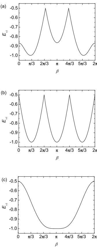
Eνλ =Wνcosβ/wν+Wλsinβ/wλ (18)
of two different distortions for all pairs of values of ν and λ taken from the set
{θ, ǫ,4,5,6}. Calculating the minimum in the energy of this factor as the angles θ
and φ are varied allows us to examine the effect of varying the contribution from two different distortions for a fixed overall magnitude of distortion. We find that the results fall into four categories. Firstly, the energy of the combinations Wǫ–W6, W4–W5, W4–
W6 and W5–W6 are all independent of the mixing angle β, taking the value − √
3/2 found for the separate components {ǫ,4,5,6}. However, the same is not true for other combinations of these four directions. For ν = ǫ and λ = 4, the minimum energy is a minimum of √3 cosβ/2 and the value of Eνλ with φ = π/2 and tan 2θ = 2 tanβ,
as shown in Fig. 2(a). For ν = ǫ and λ = 5, the minimum energy is a minimum of
0 π/3 2π/3 π 4π/3 5π/3 2π -1.0
-0.9 -0.8 -0.7 -0.6 -0.5 (a)
E
0 π/3 2π/3 π 4π/3 5π/3 2π -1.0
-0.9 -0.8 -0.7 -0.6 -0.5 (b)
E
0 π/3 2π/3 π 4π/3 5π/3 2π -1.0
-0.9 -0.8 -0.7 -0.6 -0.5 (c)
[image:10.595.208.376.93.524.2]E
Figure 2. Variation inEνλ(dimensionless units) as a function of the angle β for (a)
ν=ǫ andλ= 4 (results forλ= 5 are the same if thex-axis runs fromβ =πto 3π), (b)ν =θandλ=ǫor 6, (c)ν=θ andλ= 4 or 5.
the same as in Fig. 2(a) but where the x–axis is taken to run from β = π to β = 3π
rather than from β = 0 to π.
As we have already found that the results for a distortion in the direction θ are different to those in the other four directions we have considered, it is not surprising that the results when a θ–type distortion is mixed with a distortion in another direction are also different. For combinations ν = θ and λ = ǫ or 6, the minimum energy for a given mixing angleβ is the minimum of {cosβ,cos(β+ 2π/3),cos(β+ 4π/3)}, as shown in Fig. 2(b). The remaining cases are those of ν =θ and λ = 4 and 5. Here, the result is the minimum root of Eνλ with tan 2θ = 2 tanβ/
√
One feature of all of our results is that the energy change due to a distortion of magnitude w always lies between −w/2 and −w. The maximum energy change of −w
occurs for aθ–type distortion withwθ negative, as well as for certain other combinations
of our basic distortion directions. Similarly, the smallest energy change for a fixed magnitude of distortion w occurs for a θ–type distortion with wθ positive and other
combinations of directions.
The results above show that the topology of the APES when uniaxial distortions are applied is rather complex. However, this is not obvious without a detailed examination of the potential energy terms. Linear JT coupling alone produces a trough of equal minimum-energy points that can be mapped onto the surface of a two-dimensional sphere [14]. However, as we have seen, the effect to the sphere of different symmetry-lowering distortions are far from equivalent.
4. Energies of rovibronic states
To understand how theT⊗hJT system behaves under a symmetry-lowering distortion, we have to evaluate the total energy of the system. In general, this can be written as
Eh =
R
Ψ′
g(θ
′
, φ′
γ′
)HΨg(θ, φγ)dΩdΩ
′
R
Ψ′
g(θ
′
, φ′
γ′
)Ψg(θ, φγ)dΩdΩ′
(19)
where Ψ′
gand Ψg are the total wave functions on the LAPES given by Eq. (10), evaluated
at different points on the trough of minimum-energy points, and dΩ = sinθdθdφ and
dΩ′
= sinθ′
dθ′
dφ′
are elements of volume. The numerator and denominator are therefore both four dimensional integrals.
In order to display the results, it is convenient to define a coupling constant
KH = kH
p
~/µωH, which has dimensions of energy. Also, in order to distinguish the
effects of the additional distortion from the effect of the JT coupling alone, rather than consideringEhalone it is more useful to look at the term (Eh+EJ T)/~ωH where [14, 21] EJ T =KH2/(2~ωH) is the JT energy, i.e. the energy of the lowest point on the LAPES
when no additional distortion is present.
In this paper, we will only consider the ground vibrational state with different rotational levels, although the calculations can be extended to higher vibrational states. In this case, we can extract out the zero-point energy for zero vibronic coupling and write
Eh+EJ T
~ωH = 5 2 +
3K2
H
4 I(KH, w), (20)
with
I(KH, w) =
R
Z3e3K
2 H
4 (Z
2−
1)eim(φ′−φ)
ψR′ ψRdΩdΩ
′
R
Ze
3K2 H
4 (Z
2−
1)eim(φ′−φ)
ψ′
RψRdΩdΩ′
−1 (21)
for a given rotational state. Z is the electronic overlap between two points on the trough given by:
ψ′
RandψRare the rotational wave functions at points (θ
′
, φ′
, γ′
) and (θ, φ, γ) respectively.
I(KH, w) can be evaluated for specific values of m.
As an alternative to the calculation above, low-lying energy levels can be found numerically using a recursive Lanczos technique. [23, 24, 25, 26, 27] An advantage of this method is that it automatically includes both rotational and vibrational excitations. However, applying this technique to our system brings technical problems. To avoid degenerate ‘repeated’ eigenvectors, the number of starting vectors must be set to fifteen or more, but when this is done computational problems arise. We will not consider this method any further in this paper.
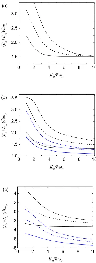
4.1. Distortion in the θ direction
First of all we will consider results for the rotational states associated with the ground vibrational state in the limit when theθ-type distortion tends to zero in order to confirm that our method gives results consistent with previous work. In this limit, we expect to obtain states which are degenerate at an energy of 1.5~ωH in strong JT coupling, representing the presence of three vibrations and two (pseudo)rotations. In zero JT coupling, we expect energies of 2.5~ωH, 3.5~ωH, 4.5~ωH etc, [21] corresponding to a five-dimensional harmonic oscillator. Each curve will have a degeneracy l = 2m+ 1, where l is odd, such that the lowest curve is for l = 1, the next curve for l= 3 etc.
For any given value of m, we can calculate rotational levels for the zero distortion case using our θ–type rotational wave functions by setting the distortion to zero. Fig. 3(a) shows the value of (Eh+EJ T)/~ωH for the first three rotational states (n = 0,
1 and 2) as calculated using either the wave functions appropriate to positive wθ and
with m= 1, or using the wave functions appropriate to negative wθ and with m= 0. It
can be seen that the results do indeed show the behavior that we expect in this limit. Note that results have not been given for KH/~ωH < 1 as the wave functions are not
appropriate for weak JT couplings. However, our results forKH/~ωH = 1 are consistent
with results for states tending to the expected limits of 2.5~ωH, 3.5~ωH and 4.5~ωH as
KH →0.
Next we consider the effects of a θ–type distortion. This will lift the m-fold degeneracy of the rotational levels. Figs. 3(b) and 3(c) give results for the lowest three rotational levels (n= 0 to 2) of the setm = 0 forwθ <0, and the setm= 1 forwθ >0.
In the latter case,m =−1 gives identical results tom= 1. Fig. 3(b) gives the results for a weak distortion of|wθ|= 0.5~ωH, and Fig. 3(c) gives the results for a strong distortion
of |wθ|= 5~ωH. As expected, the results with a distortion are lower than those with no
distortion. Furthermore, the lowering forwθ<0 is approximately twice the lowering for wθ > 0. This is also expected from the potential Ueff, which shows that the minimum
is lowered twice as much for a negative distortion as it is for a positive distortion of the same magnitude. This result is easiest to observe in Fig. 3(c) where the effects of the distortion are much larger than in Fig. 3(b).
0 2 4 6 8 10 1.5
2.0 2.5 3.0 (a)
(
E
h
+
E
J
T
)
/
H
K H
/ H
0 2 4 6 8 10
1.0 1.5 2.0 2.5 3.0 3.5 (b)
(
E
h
+
E
J
T
)
/
H
K H
/ H
0 2 4 6 8 10
-8 -6 -4 -2 0 2 4 (c)
(
E
h
+
E
J
T
)
/
H
K H
[image:13.595.211.376.94.545.2]/ H
Figure 3. (Color online) Plot of (Eh+EJT)/(~ωH) versusKH/~ωH for a distortion
applied in theθdirection for (a) no symmetry-lowering distortion (wθ →0), (b) weak
distortion (wθ=±0.5~ωH), and (c) strong distortion (wθ=±5~ωH). In all plots, the
solid lines are rotational levelsn= 0, the dashed lines are forn= 1 and the dot–dash lines are forn = 2. The lowest three (blue) lines for KH/~ωH = 10 are the m = 0
levels for negativewθ, and the highest three (black) lines are the m =±1 levels for
distortions can be explained by examining Ueff, the absolute values of the energies
can not be explained without performing the detailed calculation. Also, Ueff does not
explain why the results for different values of n with a distortion do not reach the same value as each other in strong JT coupling until much larger values of KH/~ωH
than with no distortion. These features can be attributed to changes in the form of the rotational wave function. The effect of the distortion is to select out a circle of minimum-energy points characterized by the angle φ for a fixed value of θ (namely θ = π/2 for
wθ > 0 and θ = 0 for wθ < 0), whereas for no distortion all values of the angle θ
also result in the minimum energy. Therefore one of the two pseudorotations for zero distortion is converted into a vibration with a strong distortion. As a consequence, there is a significant change in the rotational wave function as the strength of the distortion increases, from one which is not localised in θ to one which is. In the strong distortion limit, the wave function is really one for a vibration in this coordinate rather than a function for a rotation.
The energies in Fig. 3 were calculated by integrating over all points {θ, φ} that form the trough of minimum-energy points with no distortion. However, as θ is fixed at a specific value for a strong distortion, a good approximation to the energy for large distortions can be obtained if we fix θ to this value and only integrate over φ. This reduces the integrals from four dimensions to two. When this is done, we find that the results are very similar to those with the full four-dimensional integrals. For example, results for |wθ| = 5~ωH only differ by ≈ 0.01~ωH. Hence a good approximation to the
energies for a strong distortion can be found by integrating over two dimensions only.
4.2. Distortion in directions {ǫ,4,5,6}
As mentioned in Section 3.2, the minimum inUeff for a distortionWν is at the same value
for all directions ν =ǫ,4,5 and 6, and also at the same value irrespective of the sign of
wν. As a consequence, we expect the energies of the rovibronic states to be the same
for all of these cases. In fact, this provides a useful check on the method of calculation. From our calculations, we find agreement to at least 10−5
~ωH for distortions wν with
the different values of ν above, and for equivalent positive and negative distortions. As mentioned previously, only states with m even are allowed for the w4 and w5
-type strains, whereas m must be odd for wǫ and w6-type strains. Fig. 4 shows the
average energy of the lowest three rotational states of the lowest allowed value of m, namely for m =±1 for ν =ǫ or 6 and m= 0 for ν = 4 or 5. The upper (dashed blue) results are for a weak distortion of |wν| = 0.5~ωH, and the lower (solid black) results
are for a strong distortion of |wν|= 5~ωH. As expected, Fig. 4 shows that the effect of
a stronger distortion is larger than that of a weaker distortion.
For a strong distortion in the θ direction, we found that a good approximation to the energiesEh can be obtained by integrating over the angles that define the
0 2 4 6 8 10 -4
-3 -2 -1 0 1 2 3
(
E
h
+
E
J
T
)
/
H
K H
[image:15.595.215.374.96.224.2]/ H
Figure 4. Plot of (Eh +EJT)/(~ωH) versus KH/~ωH for a distortion wν where
ν =ǫ,4,5 or 6. The lower (solid black) curves are the lowest three energies for the lowest allowed value ofmandwν/~ωH=±5, and the upper (dashed blue) curves are
the corresponding energies forwν/~ωH=±0.5.
evaluate any integrals at all.
4.3. Comparison of different directions of distortion
We can investigate the effect of different distortions further by plotting results at a fixed coupling constant KH as a function of the magnitude of the distortion. Fig. 5 shows
results for KH/~ωH = 10. The solid line is for wθ positive, the dot-dashed line is forwθ
negative, and the dashed line is for |wν|/~ωH with ν =ǫ,4,5 or 6.
0 1 2 3 4 5 6 7
-8 -6 -4 -2 0 2
(
E
h
+
E
J
T
)
/
H
w / H
Figure 5. Plot of (Eh+EJT)/(~ωH) versus |wν|/~ωH for a distortion wν where
ν=ǫ,4,5 or 6. The solid curve is forwθpositive, the dot-dash line is forwθ negative,
and the dashed line is for|wν|/~ωH withν =ǫ,4,5 or 6.
[image:15.595.217.373.479.608.2]the trough. When a smallθ-type distortion is introduced, a circle of points on this sphere of minimum-energy points will become lower in energy than the other points, producing a shallow one-dimensional trough. One of the two pseudorotations will then become a hindered rotation, whereby a distortion still rotates but there is a preference for a particular distortion. As the strength of the distortion increases further, the hindered rotation will turn into a vibration about the minimum-energy point. However, other points on the APES will still influence the overall motion at these strengths. When the distortion becomes very strong, the motion will consist entirely of four vibrations and a pseudorotation. Further increases in the strength of the distortion lower the energy of the one-dimensional trough, but will not alter which points contribute to the motion.
When a small distortion in any of the directions ǫ, 4, 5 or 6 is introduced, a single point on the sphere of minimum-energy points will become lower in energy than the other points, producing a shallow potential well. Both of the pseudorotations will become hindered rotations, which turn into vibrations as the strength of the distortion increases further. Further increases in the strength of the distortion lower the energy of the potential well but, as with the θ-type distortion, will not alter which points contribute to the motion.
As a consequence of the above interpretation, we expect curves of energy against the strength of the distortion to become linear for strong distortions in any direction, with a negative gradient (to indicate that increasing the distortion strength lowers the energy) whose magnitude is closely related to the value of the energy lowering due to the distortion terms. From Section 3.3, we can see that this would predict gradients of −0.5 and −1 for positive and negative θ–type distortions respectively, and of −√3/2 ≈ −0.866 for an ǫ–type distortion. Fig. 5 shows that for strong distortions, the variation in energy is indeed linear, with gradients of−0.485,−1.285 and −0.588 for the three cases above respectively. This indicates that, for sufficiently large distortions, there is indeed a correlation between the gradients and the energy lowering due to the distortion terms.
5. Conclusion
In this paper, we have examined a linear T ⊗ h JT system subject to an additional symmetry-lowering distortion that can be written in terms of the electronic operators
σλ used to describe the intramolecular JT interaction. Physically, this situation could
represent a single C−
60 ion subject to an external stress. However, a situation which
is likely to be of much greater practical importance is a cluster or continuous solid of interacting C−
60 ions, such as found in the AC60 alkali-doped fullerides (where A is an
alkali metal). In a molecular field approximation, the effect on a given C−
60 ion of
co-operative JT interactions with other C−
60 ions can be modelled using such terms. The
co-operative interactions will result in real distortions of the icosahedral (Ih) cage of the
C60 molecule to a lower symmetry.
surfaces, where there is the possibility of transferring some of the unique properties of C60 to a solid interface. This could have important technological implications relating
to coatings and other surface modifications [28]. Being able to control the properties of organic materials leads to the possibility of exploitation in future nanostructured devices, with potential applications ranging from electronics to medicine [29]. In general, the interaction of a C60 anion with a surface will also lead to a distortion
of a system. It has therefore been suggested that surface interactions could be written (again phenomenologically), at least to a first approximation, in terms of an expansion in the σλ for anh mode, which would result in a similar symmetry-lowering distortion
to that used to describe co-operative JT effects [30]. However, to do this, the relevant operators must have a symmetry appropriate to that of both the adsorbed molecule and of the surface. This will depend upon the symmetry of the site at which the molecule is adsorbed. Therefore, it may or may not be appropriate for a real situation. If this is not the case for a given surface interaction, then it will be necessary to construct an alternative form forHsλ. Nevertheless, an analysis similar to that used here could then
follow.
The results of our calculations give the change in energy of the vibronic states of the C−
60 ion due to the introduction of symmetry-lowering terms. It might be hoped
that the results could be predicted, at least approximately, from the rather simpler analysis of the effective potential, Ueff. However, this is not found to be the case due
to significant changes in the form of the wave function when a distortion is introduced. It is nevertheless possible to simplify the calculations for strong distortions by only integrating over angles that result in minimum-energy positions (for aθ-type distortion) or by evaluating the energy at fixed angles (for anǫ, 4, 5 or 6-type distortion).
an example of where the high symmetry produces features not seen in systems of lower symmetry. Other cases where the high symmetry produces unexpected results includes the H⊗h JT system, where non-simple reducibility of the product H⊗H can result in a singlet ground state rather than the expected five-fold state [32, 33].
References
[1] Gunnarsson O. Rev. Mod. Phys., 69:575, 1997. [2] Haddon R C. Accounts Chem. Res., 25:127–133, 1992.
[3] Aldersey-Williams H. The most beautiful molecule: The discovery of the BuckyBall. John Wiley and sons, New York, 1995.
[4] Shi W, Zhou W, Cao Y, Li B, Zhang Z, and Teng Y. J. Mol. Struct., 546:11–15, 2001.
[5] Sundar C S, Gupta R, Premila M, Bharathi A, Hariharan Y, and Sood A K. J. Phys. Chem. Solids, 63:1639–1646, 2002.
[6] Lappas A, Kosaka M, Tanigaki A, and Prassides K. J. Am. Chem. Soc., 117:7560–7561, 1995. [7] Fally M and Kuzmany H. Phys. Rev. B, 56:13861, 1997.
[8] Chauvet O, Oszl`anyi G, Forro L, Stephens P W, Tegze M, Faigel G, and J`anossy A. Phys. Rev. Lett., 72:2721–2724, 1994.
[9] Remova A A, Levashov V A, Shpakov V P, Paek U H, and Belosludov V R. Synthetic metals, 86:2391–2392, 1997.
[10] Blank V D, Buga S G, Serebryanaya N R, Dubitsky G A, Sulyanov S N, Popov M Yu, Denisov V N, Ivlev A N, and Mavrin B N. Phys. Lett. A, 220:149, 1996.
[11] Ceulemans A, Chibotaru L F, and Cimpoesu F. Phys. Rev. Lett., 78:3725–3728, 1997.
[12] Stephens P W, Mihaly L, Lee P L, Whetten R L, Huang S M, Kaner R, Deiderich F, and Holczer K. Nature, 351:632, 1991.
[13] Dresselhaus M S and Dresselhaus G. Annu. Rev. Mater. Sci., 25:487–523, 1995.
[14] Chancey C C and O’Brien M C M. The Jahn-Teller effect in C60and other icosahedral complexes.
Princeton University Press, Princeton, 1997.
[15] Kaplan M D and Vekhter B G. Cooperative phenomena in Jahn-Teller crystals. Plenum Press, New York, 1995.
[16] Dunn J L. Phys. Rev. B, 69:064303, 2004.
[17] Feiner L F. J. Phys. C: Solid State Phys., 15:1495, 1982.
[18] M. C. M. O’Brien. The energy-level structure of a jahn-teller system strongly coupled to many modes of vibration. Journal of Physics C: Solid State Physics, 16(1):85–106, —1983—. [19] Dunn J L and Bates C A. Analysis of thet1u⊗hgjahn-teller system as a model for c60molecules.
Phys. Rev. B, 52(8):5996–6005, 1995. [20] O’Brien M C M. Phys. Rev. B, 53:3775, 1996.
[21] Dunn J L, Eccles M R, Liu Y M, and Bates C A. Phys. Rev. B, 65:115107, 2002.
[22] Abramowitz M and Stegun I A. Handbook of mathematical functions. Dover, New York, 1964. [23] Bevilacqua G, Martinelli L, and Pastori G P. Revista Mexicana de F´ısica, 44:15, 1998.
[24] Van Loan C F and Golub G H. Matrix Computations. John Hopkins University Press, Baltimore, 1996.
[25] Simon H D. Linear Algebra and its Applications, 61:101, 1984. [26] Parlett B N and Scott D S. Math. Comput., 33:217, 1979.
[27] Bai Z J, Day D, and Ye Q. Siam J. Matrix Anal. Appl., 20:1060, 1999. [28] Bonifazi D, Enger O, and Diederich F. Chem. Soc. Rev., 36(2):390–414, 2007. [29] Zhang E Y and Wang C R. Curr. Opin. Colloid Interface Sci., 14(2):148–156, 2009.
The Jahn-Teller effect Advances and Perspectives, Springer Series in Chemical Physics, page In Press. Springer-Verlag, 2009.
[31] Moujaes E A, Dunn J L, and Bates C A. J. Mol. Struct., 838:238–243, 2007.
[32] Moate C P, O’Brien M C M, Dunn J L, Bates C A, Liu Y M, and Polinger V Z. Phys. Rev. Lett., 77(21):4362–4365, 1996.