Quantum correlations in and beyond quantum entanglement in bipartite continuous variable systems

QUANTUM CORRELATIONS IN AND BEYOND QUANTUM

ENTANGLEMENT IN BIPARTITE CONTINUOUS VARIABLE

SYSTEMS

Richard Tatham

A Thesis Submitted for the Degree of PhD

at the

University of St. Andrews

2012

Full metadata for this item is available in

Research@StAndrews:FullText

at:

http://research-repository.st-andrews.ac.uk/

Please use this identifier to cite or link to this item:

http://hdl.handle.net/10023/3060

This item is protected by original copyright

Quantum correlations in and beyond quantum

entanglement in bipartite continuous variable

systems

Richard Tatham

School of Physics and Astronomy

This thesis is submitted in partial fulfilment for the degree of

PhD

at the

University of St Andrews

Abstract

This thesis explores the role of non-classical correlations in bipartite

con-tinuous variable quantum systems, and the approach taken is three-fold.

We show that given two initially entangled atomic ensembles, it is

pos-sible to probabilistically increase the entanglement between them using a

beamsplitter-like interaction formed from two quantum non-demolition (QND)

interactions with auxiliary polarised light modes. We then develop an elegant

method to calculate density matrix elements of non-Gaussian bipartite

quan-tum states and use this to show that the entanglement in a two mode squeezed

vacuum can be distilled using QND interactions and non-Gaussian elements.

Secondly, we introduce a potential new measure of quantum

entangle-ment in bipartite Gaussian states. This measure has an operational meaning

in quantum cryptography and provides an upper bound on the amount of a

se-cret key that can be distilled from a Gaussian probability distribution shared

by two conspirators, Alice and Bob, given the presence of an eavesdropper,

Eve.

Contents

Contents iii

Acknowledgements v

Publications vi

Conference Presentations vii

I

Introductory Material

1

1 Introduction 2

2 Continuous Variable Systems 5

2.1 Introductory quantum optics . . . 5

2.2 Phase space quasiprobability distributions . . . 13

2.3 Gaussian States . . . 16

2.4 Summary of Chapter 2 . . . 21

II Quantum Entanglement

22

3.2 Characterising Bipartite Entanglement . . . 24

3.3 Separability and Non-separability Criteria . . . 28

3.4 Entanglement Distillation and Bound Entanglement . . . 30

3.5 Entanglement Measures . . . 32

3.6 Summary of Chapter 3 . . . 37

4 Entanglement Distillation in Macroscopic Atomic Ensembles using effective beamsplitter approximation 38 4.1 Motivation . . . 38

4.2 The system and interactions . . . 39

4.3 A beamsplitter interaction between light and an atomic ensemble . . . 41

4.4 Entanglement distillation of two atomic ensembles . . . 44

4.5 Modelling Detector Inefficiencies . . . 48

4.6 Summary of Chapter 4 . . . 50

5 Entanglement Distillation with QND Hamiltonians 52 5.1 Motivation . . . 52

5.2 Protocol I . . . 53

5.3 Protocol II . . . 57

5.4 Summary of Chapter 5 . . . 60

6 Gaussian Intrinsic Information 63 6.1 Motivation . . . 63

6.2 Intrinsic Information in qudit systems . . . 66

6.3 Introducing Gaussian Intrinsic Information . . . 67

6.4 Properties . . . 70

6.5 Summary of Chapter 6 . . . 74

III Beyond Entanglement

75

7.2 The Koashi-Winter Relation . . . 79

7.3 Physical Interpretation of the Quantum Discord . . . 80

7.4 Extension to Gaussian states . . . 83

7.5 Alternative non-classicality indicators . . . 85

7.6 Summary of Chapter 7 . . . 87

8 Extension of MID and AMID to continuous variables 88 8.1 Measures of quantum correlations in Gaussian states . . . 88

8.2 Measurement Induced Disturbance of two mode Gaussian states . . . 89

8.3 Gaussian AMID of two mode Gaussian states . . . 92

8.4 Comparison between nonclassicality measures for Gaussian states . . . 96

8.5 Nonclassicality versus entanglement . . . 99

8.6 Summary of Chapter 8 . . . 102

9 Non-classical correlations in the continuous variable Werner state 103 9.1 The continuous variable Werner state . . . 104

9.2 Two mode squeezed vacuum and pure vacuum mixture: µ= 0 . . . 104

9.3 General case . . . 111

9.4 Partially transposed CV Werner state . . . 114

9.5 Summary of Chapter 9 . . . 117

IV Concluding Remarks

118

10.2 Summary . . . 123

A Multivariable Hermite Polynomials 125

B Symplectic Diagonalisation of two-mode Gaussian states in standard form 127

C Comment on measurements of Alice and Bob in Gaussian Intrinsic

infor-mation 130

D Reduction to covariant Rank-One POVMs in the analysis of Gaussian

Ame-liorated Measurement Induced Disturbance 131

Acknowledgements

There are several people that I would like to thank for supporting me during this thesis. Firstly, I would like to thank my supervisor, Dr Natalia Korolkova for her support and guidance through-out my time at St Andrews. I would like to thank my collaborators at the University of Not-tingham, Dr Gerardo Adesso and Davide Girolami for the fantastic work that they have done. I owe a thank you to Dr David Menzies who assisted me greatly in my first year. Most of all, I would like to thank Dr Ladislav Miˇsta from Palack´y University who has proven how patient a person can be when asked lots of stupid questions, and has provided a lot of direction. He has become a true friend and a fantastic collaborator. Finally, I would like to thank Anastasija and my family for indulging my non-stop talking about quantum information.

Publications

The following is a list of publications that have arisen as a result of the research of this thesis. They are presented in chronological order and are referred to throughout the thesis.

[I] R. Tatham, D. Menzies and N. Korolkova,

An approximate beamsplitter interaction between light and atomic ensem-bles,

Phys. Scr. T143, 014023, (2011)

[II] L. Mista, R. Tatham, D. Girolami, N. Korolkova and G. Adesso,

Measurement-induced disturbances and non-classical correlations of Gaus-sian states,

Phys. Rev. A83, 042325, (2011)

[III] R. Tatham and N. Korolkova,

Entanglement concentration for two atomic ensembles using an effective atom-light beamsplitter,

J. Phys. B: At. Mol. Opt. Phys. 44, 175506, (2011)

[IV] R. Tatham, L. Mista, G. Adesso and N. Korolkova,

Nonclassical correlations in continuous-variable non-Gaussian Werner states,

Phys. Rev. A85, 022326, (2012)

[V] R. Tatham and N. Korolkova,

Entanglement concentration with quantum non demolition hamiltonians, ArXiv:1111.4557. Submitted to Phys. Rev. A

Manuscripts in Preparation

• L. Miˇsta and R. Tatham,

Gaussian Intrinsic Information

June 2012

• R. Tatham, N. Quinn and N. Korolkova,

The dispersion of quantum correlations in the distribution of entanglement via separable ancilla

May 2012

Conference Presentations

The following is a list of conferences in which I have taken part.

1. 16th _{Central European Workshop on Quantum Optics (CEWQO 2009), Turku, Finland,} 2009, Poster Presentation.

2. 11th _{International Conference on Squeezed States and Uncertainty Relations (ICSSUR} 2009), Olomouc, Czech Republic, 2009, Poster Presentation.

3. Summer School on Scalable Quantum Computing with Light and Atoms, Cargese, Corsica, 2009, Poster Presentation.

4. Invited seminar at University of Nottingham, United Kingdom, 2010, Oral Presentation.

5. 17th _{Central European Workshop on Quantum Optics (CEWQO 2010), St Andrews,} United Kingdom, 2010, Poster Presentation.

6. International Workshop on Continuous Variable Quantum Information Processing (CVQIP’10), Herrsching, Germany, 2010, Poster Presentation.

7. International Conference Photon10 QEP-19, Southampton, United Kingdom, 2010, Poster Presentation.

8. Quantum Information Scotland (QUISCO), Scotland, 2011, Oral Presentation.

9. Rank Prize Funds Symposium, Grasmere, United Kingdom, 2011, Oral Presentation.

10. International Conference on Quantum Information Processing and Communication (QIPC’11), Zurich, Switzerland, 2011, Poster Presentation.

11. Participant in Quantum Discord Workshop, Singapore, 2012

Research visits

• Palack´y University, Olomouc, Czech Republic, April-May 2011

• Centre for Quantum Technologies, Singapore, January 2012

Part I

Introductory Material

Chapter

1

Introduction

The development of quantum theory can be regarded as the greatest revolution of the 20th century, sweeping away the determinism of the preceding centuries and replacing it with inherent quantum uncertainty. In the years since, quantum mechanics has proven to be an undeniably successful theory. It began its journey explaining black body radiation and the photoelectric effect, and has since been used to explain the behaviour of elementary particles, chemical bonds, and the structural properties of crystals. The theory of light has not escaped the vast scope covered by quantum mechanics, with Maxwell’s infamous equations now viewed as statistical truths.

One of the strangest things that quantum systems are capable of is to follow non-local dynamics [1] and to become correlated in non-local ways [2], unthinkable in the classical realm. Such phenomena are now regularly observed in laboratories worldwide, and any physical theories that claim to dispel non-locality are seen as increasingly quixotic.

Consider two people, Alice and Bob, separated by lightyears but sharing two particles from a common source. Each perform space-like separated experiments. That is, the experiments take a short time compared to the time period required for light to propagate from Alice and Bob and vice versa. Alice’s experiment finishes before she could receive any classical communication from Bob, and Bob is likewise ignorant of Alice’s experimental results. Only much later on, after Alice and Bob communicate classically, does it become apparent that their results are, in fact, correlated. Whatever the experimental results of one party, the other’s have been non-locally influenced. These results should perhaps be expected to be correlated - after all, the two particles came from the same source. However, the beauty lies in the fact that Alice and Bob could choose to perform any measurement that they wished on their respective particles and the measurements of the other would be influenced. If they were to instead use classical objects then such correlations would require superluminal communication. This observation is at the core of all investigations intoquantum entanglement.

That non-local correlations can exist at all without conflicting with Einstein’s relativity, is possible only because all measurement outcomes are probabilistic in nature. Quantum mechanics is indeterministic, and as such can peacefully coexist with relativity. In fact, Aharanov and Shimony [3] have independently posited that relativity and non-locality are the only axioms required to uniquely define quantum mechanics amongst the myriad of other physical theories.

The indeterminacy enters at the most fundamental level - when we ask what is meant by a quantum state. Regardless of whether one holds to the Copenhagen interpretation, countless experiments have suggested that atoms may act like waves and light may act like a stream of particles. Add into the mix Heisenberg’s uncertainty principle, in which after one measurement a second observable would give unpredictable results, and it is easy to see why there are so many interpretational traps to fall into. In the words [4] of Stephen Hawking: “Even God is bound by the uncertainty principle and cannot know position and velocity. He can only know the wavefunction.”

The pragmatic approach is to sidestep the question and introduce a definition of a quantum state based on axiomatic principles that are born out in experiments. A quantum state ˆρis a positive semi-definite, Hermitian matrix1_{, inhabiting a Hilbert space such that Tr [ ˆρ] = 1. This}

1_{The “hat” above theρis used to denote an operator, as the density matrix can be viewed as an operator}

last condition is to ensure that any probability distribution resulting from measurements of the quantum state normalise. At the first hurdle, it appears that the quantum theory is unclear, as there is no way that a single measurement on a single quantum object can yield an entire probability distribution. It is, then, implied that ˆρdenotes the statistical properties of an entire ensemble of identical quantum objects2_.

The only other important comment to be made on this is that a density matrix may be used to describe multiple systems. Two entirely statistically separate entities ˆρ1and ˆρ2can have their density matrices combined as ˆρ= ˆρ1⊗ρˆ2in a larger Hilbert space. Thus, we can largely remove any analysis of quantum correlations from specific experimental settings and instead analyse the properties of the abstract ˆρ. Correlations between subsystems will be contained within the density matrix.

If a quantum state is examined entirely without any environmental interactions, i.e. we have complete statistical knowledge of the system, then the state is said to bepure. However, if there are interactions with any system not accounted for in ˆρ, then ˆρis said to form amixed state. A mixed state is not a fundamental object. A mixed state is simply a sign of ignorance on the behalf of the researcher. If we have initially a pure state in a laboratory, but it is not closed off from the elements, it is clear that information will be lost to the environment.

Traditionally, one could verify the purity of their quantum state by checking that Tr

ˆ

ρ2

= 1. Another tool, much used in quantum information theory, is the von-Neumann entropy [6]

S( ˆρ) =−Tr [ ˆρlog ˆρ] (1.1) where the definition is understood in terms of the eigenvalues of ˆρ. S( ˆρ) is zero if and only if ˆ

ρis a pure state. The von-Neumann entropy shall be used extensively throughout this thesis, particularly for defining the quantum mutual information that captures the total correlations between two subsystems ˆρA and ˆρB that make up the larger ˆρAB

Iq( ˆρAB) =S( ˆρA) +S( ˆρB)− S( ˆρAB) (1.2) where ˆρA= TrB[ ˆρAB].

Quantum entanglement has in recent years been identified as a potent resource in quantum communication and is now readily accepted. However, until fairly recently the physics com-munity wrongly associated all non-classical correlations with quantum entanglement. However, in 2001 [7] a crude tool, the quantum discord was established that demonstrated a different type of non-local correlation that can be formed between quantum subsystems. These non-local correlations have recently found uses in quantum computing [8], but the full repercussions have not yet been seen.

The work carried out in the pursuit of this thesis has covered a wide range of topics. In this thesis are the best results from my studies into quantum entanglement and other non-local correlations. The main focus has been on continuous variable systems (that is, density matrices in infinite dimensional Hilbert spaces) as there remains far more to be explained than in the finite-dimensional setting. Gaussian states are a special case and shall be referred to a lot.

The structure of this thesis is as follows. In Part 1, Chapter 2 gives all of the required in-formation for describing continuous variable systems. In Part 2, Chapter 3 details all of the relevant background information from entanglement theory. Chapters 4, 5 and 6 contain orig-inal work on entanglement distillation and measures. In Chapter 4 we detail a method for increasing quantum entanglement in two already entangled atomic ensembles. In Chapter 5 we explore entanglement distillation schemes using single quantum non-demolition interactions and non-Gaussian operations. In Chapter 6 we introduce a quantity that looks promising as an entanglement measure.

In Part 3, Chapter 7 contains relevant background information on quantum discord and related measurements of correlations in bipartite systems. Chapters 8 and 9 contain further original work on non-classicality indicators. In Chapter 8, we define a new non-classicality

acting in a Hilbert space.

2_{It is assumed throughout this thesis that the reader has a working knowledge of quantum mechanics and so}

measure on Gaussian states and find analytic solutions on two mode Gaussian states. In Chapter 9 we explore the quantum correlations in a simple non-Gaussian state.

The work in Chapters 4 and 5 is entirely my own. The investigation of the Gaussian Intrinsic Information in Chapter 6 is an ongoing project with Dr. Ladislav Miˇsta of Palack´y University with most work being carried out in parallel so as to make sure thare are no errors. The work of Chapters 8 and 9 has been carried out in collaboration with Dr Miˇsta and Dr Gerardo Adesso at the University of Nottingham. In both chapters, all analytic work was carried out primarily by myself and Dr Miˇsta in parallel with Dr Adesso (and in the case of Chapter 8, his PhD student Davide Girolami) performing numerical calculations. My supervisor, Dr Natalia Korolkova, has provided guidance on all projects except for the measure discussed in Chapter 6.

Chapter

2

Continuous Variable Systems

In recent years, as the drive for quantum computers and communication hurtles ever forward, more and more thought and attention has been given to how to implement quantum devices in practice. Atomic systems have long been thought of as great candidates for quantum memory and quantum repeaters [9, 10, 11]. To transmit signals, the obvious workhorse is light.

Light is a quantum object. If we shine a torch through two slits and onto a screen we see wave-like interference patterns. Light can be polarised and succumbs to diffraction and refraction. Light propagates in space and interferes with itself. Light is a wavelike object.

And yet, with suitable detectors we could consider the corpuscle nature of light in the guise of photons. Einstein was awarded the Nobel prize in 1921 for his explanation of the photoelectric effect, based on exactly that idea [12]. Light consists of particles.

The quantum nature of light has long been known. Planck’s initial treatise in 1905 asserted just that! As light is such a useful resource in quantum information theory, we here give an in-troduction to quantum optics, as the quantum language of light provides the perfect playground in which to introduce continuous variable systems.

In what follows we discuss the basics of quantum optics, as has been described in lots of excellent references [13, 14, 15, 16, 17, 18, 19, 20]. We shall begin by quantising the electro-magnetic field and demonstrating the different representations of light: quadrature states, Fock states, and coherent states. Once the basic formalism of continuous variable systems has been established, we shall introduce the quasiprobability distributions that best represent quantum states in phase space. We shall also discuss the special class of Gaussian states for which a covariance matrix formalism proves sufficient for most required calculations.

2.1

Introductory quantum optics

Quantisation of the Electromagnetic Field

Maxwell revolutionised science when he introduced his famous equations to describe the be-haviour of light. In dielectric media, an electric fieldEcauses the bound charges in the material to move, inducing a local electric dipole moment. This gives rise to an electric displacement fieldD=0Ewhere0is the permittivity of free space andis the permittivity of the material in question. In free space= 1. Magnetic fields can be described in terms of the magnetizing fieldH and the magnetic inductionB=µµ0H whereµ0 is the permeability of free space. The character µdefines the permeability coefficient of the material through which the light travels and in free space is given byµ= 1. Maxwell’s equations can be written in differential form as

∇ ·D= 0, ∇ ·B= 0, ∇ ×E=−∂B

∂t, ∇ ×H=− ∂D

∂t (2.1)

and also require the boundary conditions that the fields vanish at infinity.

Maxwell’s equations complemented Newtonian mechanics and ushered in the confident age in which it was thought that the universe operated along strictly deterministic lines. With the discoveries of Planck and Einstein at the beginning of the 21st _{century, quantum uncertainty} came to the fore. We can regard the classical fields E,D,B,H as the expectation values of quantum observables e.g. DEˆE=E. From this simple yet plausible assumption it follows that

the quantum field strengths must obey Maxwell’s equations as well, due to their linearity. By replacingE,D,B,Hin (2.1) with their hatted operator counterparts ˆE,Dˆ,Bˆ,Hˆ we describe the behaviour of the quantum fields.

As in classical electrodynamics, the quantum fields may be expressed in terms of a vector potentialA, which can be replaced with an operator ˆA.

ˆ

E=−∂Aˆ ∂t ,

ˆ

B=∇ ×Aˆ (2.2)

With this, the middle two of Maxwell’s equations are automatically satisfied. The electromag-netic field is gauge invariant so for simplicity we introduce the Coulomb gauge

∇ ·Aˆ = 0. (2.3)

This satisfies∇ ·Dˆ = 0 immediately.

By rewriting the fourth Maxwell equation in terms of ˆA and using the vector identity

∇ ×∇ ×Aˆ=∇∇ ·Aˆ− ∇2_{Aˆ, we arrive at}

∇2_{Aˆ −} 1

c2

∂2_Aˆ

∂t2 = 0. (2.4)

That is, the vector potential satisfies the wave equation. In deriving the wave equation, the speed of light in a vacuumcemerges asc= 1/õ00.

The wave nature of light implies that it is subject to the superposition principle: if two light fields interfere their amplitudes add together. This is due to the linearity of Maxwell’s equations, which in turn implies that the superposition principle holds in the quantum world. In fact, a quantum field ˆA(r, t) already contains all possible light fields, waiting to be made into reality by the measurement process.

If we were to consider the classical field A(r, t) then we could rewrite it as A(r, t) =

A(+)(r, t) +A(−)(r, t) with A(−)(r, t) = A(+)(r, t)

†

. A(+)(r, t) contains all amplitudes which vary ase−iωt_{, ω >0 andA}(−)_{(r, t) contains all amplitudes that vary ase}iωt_{. Importantly,} the complex conjugate is part of the complete set of classical waves because Maxwell’s equations are real.

In order to discretise the field variables, it is necessary to assume the field is contained in a finite spatial volumeV. The contributionsA(+)(r, t) can be expanded as

A(+)(r, t) =

∞

X

k=0

Akuk(r)e−iωkt (2.5)

where the Fourier coefficientsAk are constant as the field is free. WhenV contains no refracting materials all vector mode functions uk(r) must independently obey the wave equation (2.4). That is,

∇2₊ωk2

c2

uk(r) = 0 (2.6)

for all k and the Coulomb gauge implies that ∇ ·uk(r) = 0. As the modes form a complete, orthonormal set the condition

Z

V

u∗_k(r)uk0(r) dV =δ_k,k0 (2.7)

also applies.

In theory we could consider any solution to uk(r) that satisfied the correct conditions of

∇ ·uk(r) = 0, equations (2.6) and (2.7). For example, we could consider the plane wave solution appropriate to a cubic volumeV with length of sides given byL:

uk(r) = 1

L3/2eσe

Here,kis the wave vector,eσis the unit polarization vector (which is necessarily orthogonal to

kas∇ ·uk(r) = 0, and the dispersion relation|k|=ωk/cis obtained by (2.6). The polarisation index and wave vector are all encompassed in the mode indexk.

The quantised vector potential can take the form

ˆ

A(r, t) =

∞

X

k=0

r

~ 2ωk0

h

uk(r)e−iωktˆak+u∗k(r)e iωkt_ˆa†

k i = ∞ X k=0 r ~ 2ωkV

eσ

h

ei(k·r−ωkt)_ˆa

k+e−i(k·r−ωkt)ˆa†k

i

. (2.9)

All of the quantumness of field ˆA(r, t) is obtained by replacing the fourier coefficientsAkwith the operators ˆak and ˆa†kand imposing that they are mutually adjoint. Maxwell’s equations correctly give real values. The normalisation factor renders the operators dimensionless. Equations (2.2) indicate that the electric and magnetic fields can be quantised as

ˆ

E(r, t) =i

∞

X

k=0

r

~ωk 20

h

uk(r)e−iωktˆak+u∗k(r)e iωkt_ˆa†

k

i

(2.10)

ˆ

B(r, t) =i

∞

X

k=0

r

~ 2ωk0

h

(k×uk(r))e−iωktˆak+ (k×u∗k(r))e iωkt_ˆa†

k

i

(2.11)

As an ansatz, we consider that the quantum Hamiltonian of an electromagnetic field is given by replacing all field components with operators.

H = 1 2

Z

V

(E·D+B·H) dV →Hˆ = 1 2

Z

V

0Eˆ 2 + ˆ B2 µ0 !

dV (2.12)

By inserting (2.10) and (2.11) into (2.12) the Hamiltonian can be written as

ˆ

H = 1 2

∞

X

k=0 ~ωk

ˆ

a†_kˆak+ ˆakˆa†k

. (2.13)

By imposing the condition that the field amplitudes ˆA and ˆD at various points in space but at the same point in time are causally disconnected, and observing how the fields transform in time, it is possible to show [13] that the bosonic commutation relation for the introduced mode operators is

h

ˆ

ak,ˆa†k0

i

=δk,k0. (2.14)

The Hamiltonian (2.13) can then be rewritten as

ˆ

H =1 2

∞

X

k=0 ~ωk

ˆ

a†_kˆak+ 1 2

. (2.15)

The entire electromagnetic field can therefore be described by the tensor product state of all these quantum harmonic oscillators. Each one represents a single electromagnetic mode. The bosonic operators ˆak and ˆa†k can be considered as annihilating and creating photons respectively in modek. The photon number operator, counting the number of photons in modekis defined as

ˆ

nk = ˆa†kˆak (2.16)

An important consequence of the quantisation process is that the vacuum |0i has non-zero energy (h0|_Hˆ_{|0i>0). Due to Heisenberg’s uncertainty principle, the vacuum contains random} fluctuations. That is,|0iis a valid quantum state.

Quadrature states

In what follows we shall consider representations of a single mode, and for convenience drop the subscriptk. We begin by introducing two operators ˆxand ˆpcalled thequadrature operatorsand can be considered as the real and imaginary parts of the complex ˆamultiplied by a factor1 _of

√

2.

ˆ

x= √1

2 ˆa

†_{+ ˆa}

, pˆ=√i

2 aˆ

†_−ˆa

(2.17)

The annihilation operator can be written as ˆa = (1/√2)(ˆx+ipˆ). In quantum optics, the quadratures commonly correspond to the in phase and out of phase components of the electric field amplitude with respect to a reference phase. However, the physical representation of these constructs is not important - they can simply be thought of as conjugate “position” and “momentum” in phase space, satisfying the commutation relation

[ˆx,pˆ] =i (2.18)

(where~= 1). They have no bearing on the position and momentum of e.g. a photon, which in any case is challenging to define. They can be rotated by a unitary operatorU = exp[iφ] in phase space and still satisfy the commutation relation (2.18) in their new form

ˆ

xφ= ˆxcosφ+ ˆpsinφ, pˆφ=−xˆsinφ+ ˆpcosφ. (2.19) The phase shift can be thought of, in the quantum optics case, as shifting the reference phase mentioned previously. A phase shift ofπ/2 rotates from a position to a momentum representa-tion. The eigenstates of the quadratures, thequadrature states satisfy

ˆ

x|xi=x|xi, pˆ|pi=p|pi (2.20) and are orthogonal and complete:

hx|x0i=δ(x−x0), hp|p0i=δ(p−p0),

Z ∞

−∞

|xihx|dx=

Z ∞

−∞

|pihp|dp=1. (2.21)

The quadrature states are not physical as they require an infinite precision to define, but act as a useful mathematical trick. For a wavefunction represented by|ψiwe can define the probability amplitude in the position and momentum bases via

hx|ψi=ψ(x), hp|ψi= ˜ψ(p). (2.22)

The wavefunction|ψican be written as e.g.

|ψi=

Z ∞

−∞

|xi hx|ψidx=

Z ∞

−∞

ψ(x)|xidx. (2.23)

As a final note, position and momentum states are related by Fourier transform:

|xi= 1 2π

Z ∞

−∞

dpexp[−ixp]|pi, (2.24)

|pi= 1 2π

Z ∞

−∞

dxexp[+ixp]|xi. (2.25)

Fock states

Another useful state representation is the Fock or number state|ni, defined as the eigenstate of the number operator ˆn.

ˆ

n|ni= ˆa†ˆa|ni=n|ni. (2.26)

1_{In the literature, this normalisation factor is not unique and so the quadrature operators may sometimes be}

A ket|nitherefore represents a state ofnphotons (excitations). The annihilation and creation operator respectively lower and raise the number of photons in the mode:

ˆ

a|ni=√n|n−1i, (2.27)

ˆ

a†|ni=√n+ 1|n+ 1i. (2.28) The Fock state|nican then be thought of asnexcitations of the vacuum. That is,

|ni= ˆa

†n

√

n |0i. (2.29)

The Fock states are also orthogonal and complete:

hn0|ni=δn,n0,

∞

X

n=0

|nihn|=1. (2.30)

Importantly, equation (2.27) bounds the number of photons from below2 _{as ˆa|0i = 0. One} consequence of this is the following. If we express ˆa in terms of quadratures but replace the momentum operator ˆpwith−i∂/∂x, then it becomes apparent that

ˆ

a|0i= ˆa

Z ∞

−∞

dxψ0(x)|xi=

Z ∞

−∞

dxx+ (√∂/∂x)

2 ψ0(x)|xi= 0. (2.31) The solution of this equation is then

ψ0(x) = 1

π1/4e

−x2

2 ,

˜

ψ0(p) = 1

π1/4e

−p₂2

. (2.32)

That is, the vacuum state can be described by a Gaussian phase space distribution, due to the Heisenberg uncertainty relation. In a similar fashion, the quadrature distributions of thenth Fock state can be expressed as

ψn(x) =hx|ni=

Hn(x)

√

2n_n!π1/4e

−x2

2 _(2.33)

˜

ψn(p) =hp|ni=

Hn(p)

√

2n_n!π1/4e

−p2

2 (2.34)

whereHn is thenth Hermite polynomial.

Coherent states

As the mode functions uk(r) used to define the electric field in (2.10) form an orthonormal set, it logically follows that the eigenstates of the field follow an infinite succession of relations ˆ

ak|αki=αk|αki. The coherent state of the field as a whole then is made up of a direct product of the individual states|αki.

We consider a single mode and drop the mode indexk. The oscillator state which satisfies

ˆ

a|αi=α|αi (2.35)

is known as a coherent state or sometimes as a Glauber state after the Nobel prize winner who first considered them in mathematical detail [21, 22]. In actuality, coherent states were first mentioned by Schr¨odinger [23] (translated to English in [24]) as a response to criticisms by Lorentz that quantum mechanics did not allow for the emergence of classical behaviour in light. However, the idea is usually credited to Glauber who gave detailed accounts.

If we project both sides of (2.35) onto the brahn| and use the adjoint of equation (2.28) then we immediately attain the recursion relation√n+ 1hn+ 1|αi=αhn|αifrom which it can be seen that

hn|αi= α n

√

n!h0|αi. (2.36)

From the completeness of the Fock states it follows that

|αi=

∞

X

n=0

|ni hn|αi=e−|α|

2 2

∞

X

n=0

αn √

n!|ni (2.37)

where the normalisation hα|αi= 1 leads toh0|αi=e−|α|

2

2 . From (2.36) and (2.37) the photon number distribution is given by a Poissonian distribution as

pn =| hn|αi |2=

|α|2n

n! e

−|α|2

. (2.38)

That is, if we repeatedly count the number of photons in a coherent state we obtainnphotons with probabilitypn. On average we get as many photons as quantified by the mean value|α|2.

A similar situation arises classically, if we were to repeatedly count a number of randomly distributed classical particles. A Poissonian distribution is essentially classical in nature - a light source emitting a coherent state would yield a random spacing between photons and remain unaffected by the detection (annihilation) of a field excitation by definition. Some other photon emitting sources are allowed to have different statistics. For example, a thermal light source gives off “bunches” of photons revealing super-poissonian statistics, and the annihilation of the photon does not leave the thermal state unperturbed. Coherent states thus offer the “most classical” quantum description of light which is to be expected as they are produced, for example, as the output of a laser and so mimic the wave nature of classical light.

It is important to note that the set of coherent states is not orthogonal as they are not eigenstates of a Hermitian operator:

hβ|αi=e−|α|

2 2 −

|β|2

2 −β

∗_α

(2.39)

and so | hβ|αi |2 _{= exp[−|α−β|}2_{]. If |αi and |βi differ a lot then the overlap tends to zero} asymptotically.

Coherent states can be formulated in another useful way that highlights their properties in phase space. We introduce the unitarydisplacement operator

ˆ

D(α) = exp[αˆa†−α∗ˆa] (2.40) which has the properties [25]

TrhDˆ(α)i= TrhDˆ†(α)i=πδ(R(α))δ(I(α)) (2.41)

and

ˆ

D(α1) ˆD(α2) =e(α1α∗2+α

∗

1α2)_Dˆ_(α

1+α2). (2.42)

The displacement operator has the effect of adding a complex number α to the annihilation operator:

ˆ

D†(α) ˆaDˆ(α) = ˆa+α. (2.43) We could conceivably apply a negative displacement to a coherent state to see that

ˆ

aDˆ(−α)|αi= ˆD(−α) ˆD†(−α) ˆaDˆ(−α)|αi= ˆD(−α) (ˆa−α)|αi= 0 (2.44) and so ˆD(−α)|αi=|0iwhich implies that coherent states are simply vacuum states that have been displaced in phase space. Physically, of course, |αiand |0iare quite different, in energy if nothing else. They simply have the same quantum uncertainty as the vacuum, as noticed by Schr¨odinger in 1926 [23].

However, we can write the complex amplitudeαin terms of real and imaginary parts as

α=√1

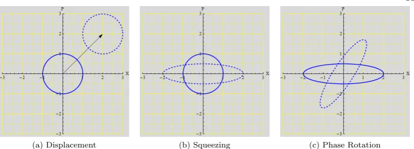
(a) Displacement (b) Squeezing (c) Phase Rotation

Figure 2.1: On a plot of position xand momentum p, a classical system could be represented by a point. In a quantum system there is inherent uncertainty. The effect of the displacement operator is to shift a distribution in phase space (Figure 2.1a). The squeezing operator (Figure 2.1b) reduces the uncertainty in one phase space variable at the expense of the other. The phase operator simply alters the quantum state’s orientation (Figure 2.1c).

Replacing (2.45) in the definition of ˆD(α) and using the Baker-Hausdorff formula [26]

eFˆ+ ˆG =e−12[F ,ˆGˆ]_eFˆ_eGˆ

=e12[F ,ˆGˆ]_eGˆ_eFˆ _(2.46)

we can write

ˆ

D(x, p) = exp

_−ip¯x¯

2

exp [ip¯xˆ] exp [−ix¯pˆ]

= exp

ip¯x¯ 2

exp [i¯xpˆ] exp [−ip¯xˆ] (2.47)

which has the effect of shifting the distributions by ¯pand ¯xin phase space e.g.

hx|αi= 1

π1/4exp

−(x−x¯)

2

2 +ipx¯ −

ip¯x¯ 2

. (2.48)

Of course, ifα= 0 then ¯x= ¯p= 0 and we have the vacuum quadrature distribution. Coherent states have the same level of uncertainty as the vacuum and are minimum uncertainty states i.e. Heisenberg’s uncertainty principle

∆x∆p≥1/2 (2.49)

is saturated for coherent states.

Minimum Uncertainty States and the Squeezing Operator

We could ask what other states saturate the bound (2.49). In fact Pauli [27] (translation [28]) used a beautifully elegant method to show that a minimum uncertainty state |φimust satisfy the equation

1 2

x

∆2_xφ(x) +

∂

∂xφ(x) = 0 (2.50)

where ∆2_{xis the variance of the position distribution. The solution to this is}

φ(x) = 1

(2∆2_xπ)1/4exp

− x

2

4∆2_x

. (2.51)

Up to displacement, minimum uncertainty states are like coherent states. However, there is another beauty to Pauli’s solution. Conceivably, the variance ∆2_{xdoes not have to equal 1/2.} That is, ∆2x and ∆2pcould differ so long as (2.49) is satisfied. The uncertainty in position

We parametrise the squeezing by parameterrand so

∆2x= 1 2e

−2r_{, ∆}2_p= 1 2e

2r _(2.52)

which can be shown to be the result of applying a unitary squeezing operator [29, 30, 31]

ˆ

S(r) = exphr 2 ˆa

†2

−ˆa2i

(2.53)

to the vacuum|0i.

Pauli’s proof showed that in fact all minimum uncertainty states are Gaussian and can be thought of as displaced, squeezed, vacuum states in phase space i.e.

|φi= ˆD(α) ˆS(r)|0i, (2.54) which encompasses the vacuum trivially and all coherent states. A minimum uncertainty state would have a position quadrature distribution of

φ(x) = 1

π1/4e r/2_exp

"

−e2r(x−x¯)

2

2 +ipx−

ip¯x¯ 2

#

. (2.55)

We can consider the effect of the squeezing operator on the vacuum in more detail by normally ordering it. Define ˆK+ = ˆa†/2

2

, ˆK− = (ˆa/2)

2

, ˆK0 = (ˆn+ 1/2), which have commutation relations

h

ˆ

K−,Kˆ0

i

= 2 ˆK−,

h

ˆ

K+,Kˆ0

i

=−2 ˆK+,

h

ˆ

K−,Kˆ+

i

= ˆK0. (2.56) The squeezing operator can then be written as

ˆ

S(r) =erK+ˆ −rKˆ−_=ef(r) ˆK+_eg(r) ˆK0_eh(r) ˆK−_{. (2.57)}

Following a method demonstrated elsewhere [32, 33, 34], if both sides of (2.57) are differentiated with respect torand multiplied on the right by ˆS−1_{(r) then the result is}

ˆ

K+−Kˆ− =f0(r) ˆK++g0(r)ef(r) ˆK+Kˆ0e−f(r) ˆK+ +h0(r)ef(r) ˆK+_eg(r) ˆK0_Kˆ

−e−g(r) ˆK0e−f(r) ˆK+. (2.58)

By applying the operator identity

eFˆGeˆ −Fˆ= ˆG+hF ,ˆ Gˆi+ 1 2!

h

ˆ

F ,hF ,ˆ Gˆii+· · · (2.59) and equating operators on each side of the equals sign in (2.58), some differential equations are found. These are

f0(r)−2g0(r)f(r) +h0(r)f2(r)e−2g(r)= 1, (2.60)

g0(r)−h0(r)e−2g(r)f(r) = 0, (2.61)

h0(r)e−2g(r)=−1, (2.62) which have the solutions

f(r) = tanh(r), g(r) =−ln [cosh(r)], h(r) =−tanh(r). (2.63) The integration constants were found by settingr= 0. Thus the squeezing operator in normally ordered form is

ˆ

S(r) =etanh(2r)ˆa

†2

e−ln[cosh(r)](ˆn+12)_e− tanh(r)

2 ˆa 2

(2.64)

which if applied to the vacuum state yields [35]

ˆ

S(r)|0i= √ 1

coshr

∞

X

n=0

_tanh(r)

2

np

(2n)!

n! |2ni. (2.65) Consequently, a squeezing operator is not passive. It alters the number of photons in a state. If we consider the energy of a given minimum uncertainty mode|φithen

hφ|Hˆ|φi=hφ|aˆ†ˆa+1

2|φi=|α| 2₊1

2 + sinh

2_{(r). (2.66)}

2.2

Phase space quasiprobability distributions

Wigner Function

With the essentials of quantum optics now explained, it is possible to consider how to represent a quantum state in phase space. On a plot of conjugate position and conjugate momentum, it would be possible to express a classical system by a single point, but quantum uncertainty renders this impossible in the quantum case as it is infeasible to observe position and momentum simultaneously and precisely. Furthermore, the very notion of a quantum state is hard to define in terms of measurements alone, and it is instead standard to carry out repeated measurements on seemingly identical systems to build up a statistical picture of a quantum object. It is, then, more sensible to consider a phase space distribution, with the singular purpose of being able to calculate observable quantities in a seemingly classical way.

Just as a particular state vector |ψi admits a quadrature wavefunction ψ(x) = hx|ψi, an operator ˆO can be described by a phase space function TrhOˆDˆ(α)i, where ˆD(α) is the displacement operator of (2.40) and satisfies a completeness relation. With this, it is possible to define acharacteristic function of a quantum density matrix ˆρas

χ(x, p) = TrhDˆ(x, p) ˆρi. (2.67)

The Fourier transform of the characteristic function yields the Wigner function first proposed by Eugene Wigner [36]:

W(x, p) = 1 (2π)2

Z ∞

−∞

χ(u, v)eiux+ivpdudv. (2.68)

The Wigner function can be written in terms ofxandpas

W(x, p) = 1 2π

Z ∞

−∞

eipqhx−q

2|ρˆ|x+

q

2idq. (2.69)

Above, for brevity, the Wigner function has been defined for a single mode only, but the extension to anN-mode Wigner functionW(x1, p1,· · · , xN, pN) is not a difficult leap of the imagination. Here we have an appropriate representation of a quantum state in phase space in the form of a Wigner function. Importantly,W(x, p) can become negative in regions or ill-behaved and so is not a true probability distribution. Also, in reality quantum position and momentum cannot be measured simultaneously to form a true probability distribution. It is a quasiprobability distribution. The Wigner function satisfies all the desirable properties that a quasiprobability distribution should have [37]. Firstly, the Wigner function has the correct marginal distributions

Z ∞

−∞

W(x, p) dx= Pr (p),

Z ∞

−∞

W(x, p) dp= Pr (x), (2.70)

where Pr signifies a probability distribution. If a density matrix ˆρis rotated in phase space by the unitary operatorU(φ) =eiφ_{, then the Wigner function transforms accordingly as}

ˆ

ρ→U(φ) ˆρU†(φ)⇒ W(x, p)→ W(xcosφ−psinφ, xsinφ+pcosφ). (2.71) The Wigner function is normalised

Z ∞

−∞

W(x, p) dxdp=1 (2.72)

By far the most outstanding property of the Wigner function is the overlap formula. For two Hermitian operators e.g. ˆρand ˆO

TrhρˆOˆi=

Z ∞

−∞

hx0|ρˆOˆ|x0idx0

=

Z ∞

−∞

hx0|ρˆ|x00ihx00|Oˆ|x0idx0dx00

= 1 2π

Z ∞

−∞

eip(q1+q2)hx−q1

2 |ρˆ|x+

q1 2ihx−

q2 2 |

ˆ

O|x+q2

2 idq1dq2dxdp = (2π)

Z ∞

−∞

Wρ(x, p)WO(x, p) dxdp. (2.73)

That is, one can calculate the expectation value of an operator ˆO acting on state ˆρby looking at the phase space distribution overlap of the two operators. The overlap formula allows for an easy change of basis. For example, if a switch to a basis |nihn| was required, then it would be only necessary to replaceWO(x, p) in (2.73) with the Fock state Wigner function

Wn(x, p) = (−1)n

π e

−x2−p2_L

n 2x2+ 2p2

(2.74)

where Ln denotes thenthLaguerre polynomial. The purity of a state can also be described by (2.73)

Tr

ˆ

ρ2

= 2π

Z ∞

−∞

W2_{(x, p) dxdp (2.75)}

and the von-Neumann entropy of ˆρis bounded by

S( ˆρ)≥1−2π

Z ∞

−∞

W2(x, p) dxdp. (2.76)

Another property of the Wigner function is that it is bounded from above,

|W(x, p)| ≤ 1

π. (2.77)

It is easy to show how a Wigner function transforms with the operators mentioned so far. In addition to the phase shift operation (2.71), the squeezing operator (2.53) and displacement operator (2.47) transform the Wigner function as

W(x, p)→ W erx, e−rp

and W(x, p)→ W(x−x, p¯ −p¯) (2.78) respectively.

Other quasiprobability distributions:

s

-parametrization

We could consider other quasiprobability distributions that have other useful properties. In particular, we could re-examine equation (2.67), defining the characteristic function as the trace of the displacement operator with the density matrix ˆρ:

χ(α) = TrhρDˆ(α)i= Trhρeαˆa†−α∗aˆi. (2.79)

Importantly, the displacement operator in (2.79) is symmetrically ordered - if the exponential was to be expanded, the operators ˆaand ˆa† _{would be combined symmetrically. By treating the}

characteristic function as a generating function, it is therefore possible to find that

D

ˆ

a†mˆan

sym

E

= Trhρˆ

ˆ

a†mˆan

sym

i

= ∂ (m+n)

∂αm_∂α∗nχ(α)_α=α∗₌₀ (2.80)

where, for example,

ˆ

a†ˆa2

sym= ˆaaˆˆa

However, one could instead use the Baker-Hausdorff formula (2.46) to rewrite the charac-teristic function in two alternative ways:

χ(α) = Tr

ˆ

ρe−|α|

2 2 eαˆa

†

e−α∗ˆa

=e−|α|

2 2 Tr

h

ˆ

ρeαaˆ†e−α∗ˆai=e−|α|

2

2 χ_N(α), (2.81)

χ(α) = Tr

ˆ

ρe|α|

2 2 e−α

∗_ˆa

eαˆa†

=e|α|

2 2 Tr

h

ˆ

ρe−α∗aˆeαaˆ†i=e|α|

2

2 χ_A(α). (2.82)

In the above, the subscriptsN andAstand for normally and antinormally ordered respectively. That is, ifχN(α) andχA(α) were to be treated as generating functions then

ˆ

a†mˆan= Trρˆˆa†mˆan= ∂ (m+n)

∂αm_∂α∗nχN(α)_α=α∗₌₀, (2.83)

ˆ

amˆa†n

= Tr

ˆ

ρˆamˆa†n

= ∂ (m+n)

∂αm_∂α∗nχA(α)_α=α∗₌₀. (2.84)

The normally ordered and anti-normally ordered characteristic functions play a special role in this thesis, but as can be seen above, one can be turned into the other by multiplying by a suitable exponential. More commonly, one defines ans-parametrised characteristic function as

χ(α;s) =χ(α)es|α|

2

2 (2.85)

which for convenience we shall write in terms of conjugate position and momentum as

χ(x, p;s) =χ(x, p)es4(x 2_+p2₎

(2.86)

The effect on the Wigner function is to convolve it with Gaussian distributions parametrised by a real parameters[38, 39]. It is also possible to define quasiprobability distributions parametrised by complex numbers [40] but that is beyond the scope of this thesis. The s-parametrised quasiprobability distributions are given by the Fourier transform of (2.86):

W(x, p;s) = 1 (2π)2

Z ∞

−∞

χ(u, v;s)eiux+ivpdudv. (2.87)

The most important cases for this thesis ares= 0,1,−1. Whens= 0, the characteristic function (2.86) is unchanged and so (2.87) reduces to the standard Wigner function.

If s = −1 then the parametrised characteristic function is the anti-normally ordered χA

and the corresponding quasiprobability distribution is known as the Q function, denoted Q. The Q function is a simple convolution of the Wigner function with the vacuum distribution

Wvac(x, p) = (1/π) exp[−x2−p2] and the result is a smooth, non-negative, normalized quasiprob-ability distribution

Q(x, p)≡ W(x, p;−1) =

Z ∞

−∞

W(x0, p0)exp[−(x−x

0₎2_−(p−p0₎2_]

π dx

0_dp0_{. (2.88)}

On comparison with the overlap formula (2.73) it is clear that the Q function simply gives the probability distribution for finding the coherent stateα= (1/√2)(x+ip).

Q(x, p) = hα|ρˆ|αi

2π (2.89)

Importantly, as will be seen in Chapter 5 the Q function acts as a generating function for density matrix elements.

For s = 1 the P function, P (also known as the Glauber-Sudarshan function [41, 42]) is obtained, and is of importance in Chapter 8. Due to theoptical equivalence theorem a density matrix ˆρcan be written as

ˆ

ρ=

Z ∞

−∞

P(x, p)|αihα|dxdp (2.90)

the P function can exhibit far worse behaviour. Not much more will be said of the P function here except that it can be very ill-behaved. After all, a pure state|ψihψ|cannot be written as a distribution of coherent states unless|ψiitself is a coherent state. In that case, the P function is simply a delta function. From this observation, the P function of a Fock state|nimust contain derivatives of a two dimensional delta function - very strange behaviour indeed.

The relationship between thes-parametrized formulae and the overlap function is

TrhρˆOˆi= 1 2π

Z ∞

−∞

Wρ(x, p;s)WO(x, p;−s) dxdp. (2.91)

2.3

Gaussian States

The primary tools for exploring quantum information theory in the continuous variable setting are the Gaussian states and Gaussian maps. Gaussian states are those states with a Gaussian characteristic function (2.67) (and hence a Gaussian Wigner function) and Gaussian maps are those transformations that turn one Gaussian state into another.

Gaussian states are of great practical relevance. The quantum vacuum, for one, is a Gaussian state, as are the coherent states|αiresulting from a displacement of the vacuum in phase space. Squeezing, phase-shifting and beamsplitter transformations, are all examples of Gaussian maps. Quite often, non-linear operations can also be approximated to a high calibre by Gaussian maps. In this Section, we shall introduce only the most relevant qualities of bosonic Gaussian states to this thesis. Consequently, a lot of fascinating areas of investigation shall not be delved into. For brilliant reviews of the basic facts of Gaussian quantum information processing, see those by Braunstein and Van Loock [43] and Ferraro [25]. For a particular focus on entanglement in Gaussian states see the PhD thesis of Adesso [44] and the review [45]. For an up-to-date overview of all Gaussian Quantum Information Theory see [46].

Definition of a Gaussian state

An N-mode Gaussian state is a state with a Gaussian Wigner function that can be written in terms of a covariance matrixγas

W(x1, p1, . . . , xN, pN) =

exph−RT −dTγ−1_(R−d)i

πN√_detγ (2.92)

where R = (x1, p1, . . . , xN, pN) T

and d = (hx1i,hp1i, . . . ,hxNi,hpNi) T

is a vector of first moments i.e. displacements. The covariance matrix is defined as

γlm =

D

ˆ

RlRˆm+ ˆRmRˆl

E

−2dldm. (2.93)

It is very important to note that definitions vary throughout the literature. The definition of the covariance matrix given above is compatible with [ˆxj,pˆk] = iδj,k. Other possibilities that frequently surface are [ˆxj,pˆk] = 2iδj,k with a factor of 1/2 appearing in (2.93) (as is used in e.g. [44] and [45]), or [ˆxj,pˆk] =iδj,k with the factor of 1/2 in (2.93), in which case the Wigner function (2.92) is altered accordingly.

Interestingly, for Gaussian states all of the s-parametrized quasiprobability distributions can be found by replacingγ in (2.92) withγs, andγs is defined by

γs=γ−s1. (2.94)

The covariance matrix is a real, 2N ×2N, symmetric matrix. To represent a feasible quantum state the only requirement is that a covariance matrix satisfy Heisenberg’s Uncertainty Principle [50] which can be expressed conveniently as

γ+iΩ≥0 (2.95)

where Ω =⊕N

j=1ω andωis given by

ω=

0 1

−1 0

. (2.96)

From the diagonal terms in (2.95) one easily derives the usual expression of Heisenberg’s un-certainty principle. From the definition (2.93), the covariance matrix of the vacuum is given by

γvac=1. All other Gaussian states can be seen as the result of Gaussian maps onγvac.

Gaussian Maps

In general, a quantum state undergoes a quantum operation [51] consisting of a linear map Ξ : ˆρ→Ξ ( ˆρ) which is completely positive and potentially trace-decreasing. More will be made of this in Chapter 3. A quantum operation is said to be a quantum channel if it is trace-preserving, and the simplest of these are reversible and represented by unitary transformations

U withU†U =1. The density matrix ˆρthen transforms asUρUˆ †. A Gaussian unitary channel therefore consists of those quantum channels that transform Gaussian states to Gaussian states. Usually the unitary can be represented byU = exp[−iHˆ] where ˆH is a Hamiltonian which is at most a second-order polynomial in the field operators ˆaand ˆa†.

As a consequence of the Stone Von-Neumann Theorem, all Gaussian unitaries acting on the Hilbert space level can be represented by a symplectic operationS on the phase space level. That is a Gaussian unitary can be identified with a matrix S that acts on the phase space variables (x,p) and is essentially defined by how the phase space variables tranform i.e.

R0 =SR. (2.97)

The matrixS must necessarily satisfy

SΩST = Ω (2.98)

to be symplectic and to preserve Heisenberg’s Uncertainty Principle. As a consequence of (2.98), detS= 1. A generic unitary Gaussian map can consist of a symplectic operation and a displace-ment. For example, if we were to displace a Gaussian state in phase space byd0 and perform a symplectic transformationS the first and second moments would transform as

d→Sd+d0, γ→SγST (2.99)

respectively.

Some of the most important transformations that have been introduced so far can be rep-resented by a symplectic operation. The squeezing operation (2.53) can be reprep-resented by

SSQ(r) =

er ₀ 0 e−r

(2.100)

and a phase space rotation can be represented by

SP H(θ) =

cosθ sinθ −sinθ cosθ

. (2.101)

The most general one mode covariance matrixγone can be represented as a result of squeezing and rotation of a thermal state in phase space and can be written as

γone= (2hni+ 1)SP H(θ)SSQ(r)γvacSSQT (r)S T

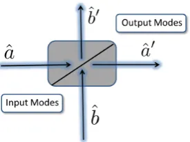
Figure 2.2: A beamsplitter is a four port optical device, taking two modes as input and releasing two modes as output. Both input modes are partially transmitted and partially reflected by the beamsplitter.

and displaced squeezed state |α, θ, ri = ˆD(α) ˆU(θ) ˆS(r)|0i although later in this thesis (e.g. Chapter 9) the rotation and squeezing are amalgamated as e.g. |α, reiθ_i.

Vitally, some very useful multimode operations are Gaussian in nature. Firstly, we have the lossless beamsplitter which takes two input modes and combines them by either transmitting or reflecting photons proportional to a transmittance coefficient T (see Figure 2.2). In the Heisenberg picture, a beamsplitter transforms the annihilation operators of the two input modes (ˆaand ˆbrespectively) as

_aˆ0

ˆ

b0

=

√

T −√1−T √

1−T √T

ˆ a ˆ b , (2.103)

and so, by taking the adjoint of equation (2.103) and representing two input Fock states|n1, n2i using equation (2.29), it can (after a lot of algebra) be shown that a beamsplitter mixes two Fock states as

|n1, n2i → 1

√ n1!n2!

n1,n2

X

k1,k2

√

T

k1

−√1−Tn1−k1 √

1−Tk2√

T

n2−k2

p

(k1+k2)!(n1+n2−k1−k2)!

× _n 1 k1 _n 2 k2

|k1+k2, n1+n2−k1−k2i. (2.104)

The total photon number is conserved, but the photons are distributed between the two output modes proportional toT. Using equation (2.104), one sees that if a single photon in each input mode is incident on a 50/50 beamsplitter, then 2 photons emerge in one output port or the other. This is the famous Hong-Ou-Mandel effect. A beamsplitter interaction between two Gaussian states can be represented by the symplectic operation

SBS(T) =

   

√

T 0 √1−T 0

0 √T 0 √1−T

−√1−T 0 √T 0

0 −√1−T 0 √T

   

. (2.105)

If we squeeze a vacuum mode inxand another mode inp, and combine both modes on a 50/50 beamsplitter (T = 1/2) then we arrive at the covariance matrix of thetwo mode squeezed vacuum

γT M SV =SBS(1/2) (SSQ(r)⊕SSQ(−r))γvac SSQT (r)⊕S T SQ(−r)

S_BST (1/2)

=

   

cosh(2r) 0 sinh(2r) 0 0 cosh(2r) 0 −sinh(2r) sinh(2r) 0 cosh(2r) 0

0 −sinh(2r) 0 cosh(2r)

   

. (2.106)

vacuum is a pure state and any two mode pure Gaussian state can be represented by covariance matrix (2.106). The Fock state representation of the two mode squeezed vacuum is

|Ψi=p1−λ2

∞

X

n=0

λn|nni (2.107)

withλ= tanh(r).

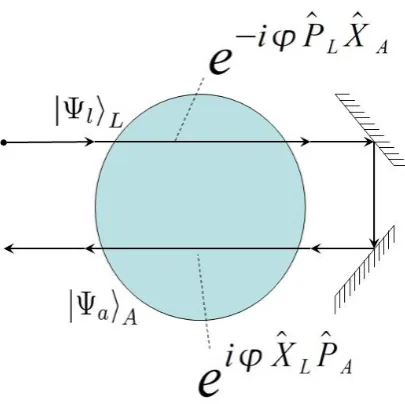
Another significant Gaussian operation is the Quantum Non-Demolition (QND) interaction. The quantum non-demolition interactions [53, 54] are well-known from quantum metrology. They are decribed by Hamiltonians of the form e.g.

ˆ

HQND=κPˆSPˆA (2.108)

whereκis the interaction strength and ˆPS/Aare the quadratures of the system/ancillary mode. The system and ancillary mode interact in such a way as to leave one quadrature component of each subsystem intact whilst phase shifting the conjugate components. In particular, in the Heisenberg picture, where the quadratures evolve via the Heisenberg equations of motion, only the position quadratures of the system and ancillary modes would be affected by equation (2.108) as the momenta quadratures commute with the Hamiltonian. Furthermore, for light it was also shown that it is possible to create a QND Hamiltonian using optical instruments such as biased beamsplitters and squeezers in combination [55].

Importantly for Chapter 5, quantum non-demolition interactions can also be represented by symplectic operations. For an interaction between a system and ancillary mode, given by

the interaction Hamiltonian ˆHint=κRˆjRˆk, the corresponding symplectic operationS (κRˆjRˆk)

QND is given by

S_QND(κXˆXˆ)=

   

1 0 0 0

0 1 −κ 0

0 0 1 0

−κ 0 0 1

   

, S(_QNDκXˆPˆ)=

   

1 0 0 0

0 1 0 −κ

κ 0 1 0

0 0 0 1

   

,

S_QND(κPˆXˆ)=

   

1 0 κ 0

0 1 0 0

0 0 1 0

0 −κ 0 1

   

, S(_QNDκPˆPˆ)=

   

1 0 0 κ

0 1 0 0 0 κ 1 0 0 0 0 1

   

. (2.109)

Symplectic analysis of Gaussian states

In 1936, Williamson [56] proved that all positive definite real matrices of even dimensions can be diagonalised by symplectic operations. For theN-mode covariance matrix γ, there always exists a symplectic transformation that puts the covariance matrix in symplectic formγν

SγST =γν =⊕Nj=1

νj 0 0 νj

, (2.110)

where ⊕ denotes the direct sum of matrices. The symplectic eigenvalues νj can be found as the eigenvalues of |iΩγ|. The determinant of any Gaussian state is easily expressed as det (γ) = Q

jν 2

j. Furthermore, for Heisenberg’s Uncertainty Principle to hold, and hence for

γ to represent a true quantum covariance matrix,νj ≥1 for allj. The symplectic diagonalisa-tion of a covariance matrix corresponds to the decomposidiagonalisa-tion of a Gaussian state into thermal modes. The covariance matrix (2.110) corresponds to the density matrix being expressed as

ˆ

ρ⊗=⊗N j=1

2

νj+ 1 ∞

X

n=0

_ν

j−1

νj+ 1

n

|nijhn|, (2.111)

where ⊗denotes the tensor product of density matrices. In this Williamson form, each mode is a Gaussian state in thermal equilibrium at a temperature Tj characterised by the average number of photons hnjiand frequency ωj. The average number is described by Bose-Einstein statistics

hnji=

νj−1

2 =

1

exp[ ~ωj

kBTj]−1

There are other important quantities relating to the symplectic spectrum{νj}. The seralian [57] is defined as the sum of the determinants of all the 2×2 submatrices ofγ and can be calculated from symplectic eigenvalues via

∆ (γ) = N

X

j=1

ν_j2. (2.113)

The invariance of ∆ for multiple modes [58] follows from the the knowledge that all symplectic operations can be decomposed as products of two-mode transformations [59] and the invariance of ∆ in the two-mode case (see [60] for proof).

The von-Neumann entropy of anyN-mode Gaussian state can easily be calculated in terms of the symplectic eigenvalues of covariance matrixγ [61]. The entropy is calculated via

S(ρ) = N

X

j=1

F(νj) (2.114)

where

F(ν) =

_{ν+ 1}

2

ln

_{ν+ 1}

2

−

_ν−1

2

ln

_ν−1

2

. (2.115)

Noticeably, the state is pure (i.e. entropy (2.114) is zero) if and only if νj = 1 for allj. The covariance matrix of apure Gaussian state satisfies

−ΩγΩγ=−ΩSSTΩSST =−ΩSΩST =−ΩΩ =1 (2.116)

whereγ can be expressed asSST _{for all pure states.}

Bipartite Gaussian States

If we were to consider that two parties, Alice and Bob, possessed a Gaussian state (ofmandn

modes respectively), the covariance matrix of the system could be expressed as

γ=

α σ

σT _β

(2.117)

where αis a 2m×2mmatrix, β is a 2n×2nmatrix and σ contains the correlations between Alice and Bob’s modes.

It would be most desirable to explore how a bipartite Gaussian state transforms under local Gaussian operations. As Gaussian maps have effects only on the level of covariances, it is possible to formulate the effect of a Gaussian map on a Gaussian state also in terms of covariances. There have been many works ([62],[63] to name a few) showing how a bipartite state transforms under a Gaussian map reducing the number of modes. Ultimately, if we were to project Bob’s modes onto a Gaussian state with covariance matrixγp, then a Gaussian operation has been performed. The result is that the covariance matrix of Alice’s modes, and their displacement in phase space, are transformed as

γ→α−σ(β+γp)−1σT, d→ 1

2σ(β+γp)

−1

d. (2.118)

The proofs given in the literature are complicated but the principle behind (2.118) is simple, and just requires the overlap formula (2.73). Consider, as an example, a map where there are no displacements i.e. we are only concerned with the transformation of the covariance matrix. Then we express

γ−1= α−σβ

−1_σT−1

− α−σβ−1_σT−1

σβ−1

−β−1_σT _α−σβ−1_σT−1

β−1_+β−1_σT _α−σβ−1_σT−1

σβ−1

!

=

A C

CT _B

The measurements of Bob’s modes (with Gaussian measurement ˆGB) can be written using the Wigner overlap formula as

TrhρˆABGˆB

i

= (2π) n

exp

−ηT AAηA

πm+n√_detγ

Z ∞

−∞

exp−ηTB B+γ− 1 p

ηB−2ηTACηB

dηB

= (2π)

n

πn

πm+n√_detγq_{det B+γ}−1

p

exph−ηTA

A−C B+γ−p1

−1

CTηA

i

(2.120)

whereηT

A= (x1, p1,· · · , xm, pm) andηBT = (xm+1, pm+1,· · ·, xm+n, pm+n). This can be thought of as a probability of projecting onto ˆGB multiplied by a Wigner function characterised by the covariance matrixγ0=A−C B+γ_p−1−1CT

−1

which, with repeated and careful use of the binomial inverse theorem

(A+U BV)−1=A−1_{− A}−1_{U B B+BVA}−1_{U B}−1

BVA−1 _(2.121)

can be put into the required form (2.118). Homodyne detection of Bob’s modes is a projection onto a pure generic state, given for a single mode in (2.102), in the limit of infinite squeezing. Heterodyning too is a Gaussian map.

In a similar way, we can also consider what happens to the covariance matrix of subsystem

A if we trace out subsystemB. Using the Wigner Overlap formula and utilising the binomial inverse theorem it is possible to show that the covariance matrix of equation (2.117) reduces to simplyα. That is, we simply cut away all other submatrices (β andσ).

Most important for this thesis is the case when Alice and Bob each possess a single mode (m=n= 1). If this is the case then there exist local symplectic operationsS1 andS2, applied asS=S1⊕S2, that transformγ into thestandard form

γ=

   

a 0 c+ 0

0 a 0 c−

c+ 0 b 0

0 c− 0 b

   

(2.122)

which can be a mixed state in general. The invariants of this standard form can be expressed as

detγ= (ab−c2₊)(ab−c2₋), (2.123) ∆(γ) =a2+b2+ 2c+c− (2.124)

and the symplectic eigenvalues are given by

ν±=

s

∆(γ)±p∆2_{(γ)−4 detγ}

2 (2.125)

2.4

Summary of Chapter 2

The standard toolbox for quantum optics has been unpacked in this chapter and proves very useful for describing continuous variable systems in general. The beauty of the language of quantum optics is that it shows, in effect, the boundary between particle and wave-like quantum objects in continuous variables. The Wigner function and other phase space quasiprobability distributions provide, for a single mode, a way to visualise a quantum state.

Part II

Quantum Entanglement